On Real-Time Accounting of Inventory Costs in the Newsvendor Model and Its Effect on the Service Level ()
1. Introduction
In contrast to deterministic demand models, such as the economic order quantity (EOQ), which assume continuous accounting of inventory costs, most stochastic periodic-review inventory models assume that inventory costs are calculated according to the inventory level at the end of the replenishment period. For example, the newsvendor problem assumes only overage and underage costs (denoted co and cu, respectively) and the optimal policy is obtained when the probability of not stocking out in a review cycle (a probability referred to as the type 1 service level) is equal to . It seems that developers of stochastic models use this cost accounting approach as a means of increasing their models’ mathematical tractability. However, when the period is not short, this accounting approach might lead to substantial loss, as is shown by Rudi et al. [1] .
Only recently have stochastic periodic review models been modified to consider the real times at which inventory costs occur within each period. Rao [2] analyzed the long-run average cost in a periodic review  model with backlogging, in which inventory-related costs accrue in continuous time. Rudi et al. [1] dealt with a similar problem and suggested an approximation formula for the optimal order-up-to level when the period length is given and demand is a Brownian motion process. Shang and Zhou [3] and Shang et al. [4] analyzed a full backlogging serial inventory system with inventory costs that accrue at evenly-spaced points within the period. To minimize the average cost per period they suggest a heuristic procedure based on calculating lower and upper bounds for the cost function.
The four papers above deal with a multi-period model and share few underlying assumptions: full backlogging of unsatisfied demand and no spoilage; holding and shortage costs that are only duration-dependent; and stationary demand process within the period. For example, Rudi et al. [1] show that, in a full backlogging system in which both holding and shortage costs are accounted for continuously, the optimal policy is obtained when the fill rate (referred to as the type 2 service level) is equal to . However, this result does not hold in the case of lost sales, in which only the holding cost is duration dependent, whereas the cost of a stock-out predominantly depends on the stock-out quantity. This case is applicable to perishable items such as fresh food and fashion items, which are mostly analyzed under the assumptions of deterministic demand and forbidden shortages (see, e.g., Avinadav and Arponen [5] ; Avinadav et al. [6] , Avinadav et al. [7] ; Herbon [8] ; Dash et al. [9] ).
The current research seeks to explore how the two different approaches to inventory cost accounting affect the solution of a periodic review model with stochastic demand. To this end, we use the classical newsvendor problem as a benchmark (Arrow et al. [10] , Hadley and Whitin [11] ), reformulate it, and solve it according to the real-time holding cost accounting within the period. Our approach, which is demonstrated in the following sections, can be extended to more elaborate periodic review inventory models, such as multi-period models with partial backlogging and spoilage, and to include lead time, duration-dependent shortage cost, fixed order cost and non-stationary inventory costs within the selling period.
The selling period is split into several equal-time epochs (see also [3] and [4] ) according to the minimal duration in which holding costs accrue (e.g., a business day, a week, etc.). The approach of splitting the selling period into epochs was previously suggested by Sen and Zhang [12] as a means of considering multiple demand classes, and by Chung et al. [13] as a means of allowing for in-season price adjustments. A common assumption, which is also assumed here, is that unsatisfied demand is lost, so that shortage leads to a loss of profits, which depends only on the stock-out quantity (and not on the duration). Actually, such a model was suggested as a direction for future research by Rudi et al. [1] , who analyzed a full backlogging inventory system, and it is applicable to many inventory systems of perishable items, such as supermarkets and fashion stores.
Although the selling period is divided into epochs to handle holding costs correctly, we assume that inventory cannot be replenished within the period, even when inventory is exhausted. This assumption is fundamental in all periodic review models and is valid for several reasons, such as fixed replenishment dates dictated by the supplier/producer (e.g., in food products) and lead-time (including production time) that is equal to or greater than the selling period (e.g., in fashion stores). In contrast to the models in [1] [4] , in which an assumption of stationary demand process is essential, our model allows for non-stationary demand. Relaxation of the assumption of stationary demand is important in order for our model to be applicable to the case of perishable items, which are characterized by deteriorating demand within their selling period due to loss of freshness and customers’ preference for fresh items (see, e.g., [5] -[8] ). Typically, in order to free up space for new or fresh items, vendors of perishable items sell all leftover units at salvage value at the end of the selling period or even distribute them for free to save scrap costs (see, e.g., Cachon and Kök [14] ). Accordingly, we analyze examples in which the expected demand in each epoch is not greater than that of its predecessor epoch. This is an extension of the deterministic negative time-effect within the selling period, used in [5] .
The main achievements of this study are 1) formulating the expected profit function for real-time holding cost accounting (in Section 2); 2) showing that the expected profit function is concave, formulating the optimality equation as the classical newsvendor formula with modified demand distribution and cost parameters, and suggesting a search algorithm to obtain the optimal order quantity (in Section 3); and 3) suggesting simple heuristics to obtain the optimal order quantity and bounds on its value (in Section 4), and evaluating their performance (in Section 5).
2. Model Formulation
We assume the standard assumptions of the newsvendor problem, where unsatisfied demand results only in loss of profit, and overage units are sold at salvage value to a secondary market. Regarding the main feature of the model, division of the selling period into epochs, we assume that the cost of holding a single item in stock is constant across epochs. On the other hand, we do not assume that demands across epochs are independent or identical. We develop the model for discrete demand to allow a point mass probability of zero demand (which characterizes inventory systems with small demand rates), and to support our numerical examples (Section 5), which assume a Poisson demand process (as is common in the literature). Extension to more elaborate models of the newsvendor problem is not complicated, and is specifically simple for models with continuous demand and with duration-dependent shortage costs.
In the rest of this paper we use the following notations:
n = the number of epochs in which holding costs are accounted for during the selling period.
dk = the demand in the kth epoch.
 = the cumulative demand in the first
  epochs (
 ).
).
 = the probability function of
 .
.
 = the cumulative distribution function (CDF) of
 .
.
mk = the mean of .
.
sk = the standard deviation of .
.
 = the quantity of an order, which is the decision variable.
 = the stock level after the first
  epochs (
 ).
).
 = the total stock during the selling period stored for an epoch (
 ).
).
h = the holding cost of an item for an epoch.
c = the purchasing cost of an item from the supplier.
r = the retail price of an item within the selling period (r > c).
s = the salvage value of an item at the end of the selling period (0 £ s < c).
 = the expected net profit, which is the objective function.
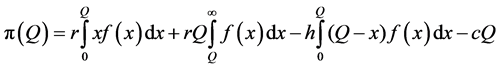
The expected profit from selling units is a function of three elements: purchase cost, revenue, and stock holding costs. Our formulations of the first two elements do not diverge from those of the standard newsvendor model: the purchase cost is cQ, and the expected revenue, which includes revenue from units that are sold within the selling period, as well as the salvage value of the remaining units, is
 (1)
(1)
where
 (2)
(2)
is the expected shortage during the first  epochs. The expression on the right-hand side of Equation (1) can be explained as follows: all purchased units yield a guaranteed revenue per unit that is equal to the salvage value
 , where the expected sales volume during the entire period (expected demand less expected shortage) yields additional revenue per unit beyond the salvage value
 .
.
The expected total stock over the whole period is
 . (3)
. (3)
Note that  replaces the commonly used “end-of-period” stock calculation, according to which the expected total stock is
 . Finally,
 . (4)
. (4)
Equation (4) fits also the continuous demand case, and as shown in Appendix A, it is a generalization of the classical newsvendor profit function, which is obtained by substituting n = 1 and s = 0.
3. The Optimal Order Quantity
The profit function in the classical newsvendor problem is known to be concave (Hadley and Whitin [11] , p. 299). The following lemma shows that this property is also valid in our model. Let  be the difference equation of the profit.
Lemma 1.  is non-increasing in
 .
.
Proof. By Equation (2),
 so that, by Equation (4),
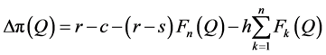 . (5)
. (5)
Since  is non-decreasing in
 , then
  is non-increasing in
 .
.
Let  be the optimal order quantity. Then, by Lemma 1, we state Theorem 1.
  is concave and
  is the smallest integer
  that satisfies
 . (6)
. (6)
Dividing Equation (6) by ,
,  is the smallest integer
  that satisfies
 , (7)
, (7)
where ,
,  ,
,  ,
,  ,
,  and
and
 . Since
  then, according to Chatfield and Theobald [15] ,
  is the CDF of a mixture
(of random variables).
Actually, the random variable X can be considered as the demand over a subinterval of the selling period; this subinterval starts at the first epoch, and its length (in epochs) is a random variable over the support  with probabilities that correspond to the cost ratios
 ,
, . Thus, by Equation (7), we conclude that considering the real-time holding cost accounting within the selling period results in the classical newsvendor optimality condition (Nahmias [16] , p. 244) with modified demand distribution and cost parameters. Specifically, the mixture
  replaces the demand over the entire period,
 ;
;  denotes now the maximal loss of profit due to lost sales (as if all sales take place immediately at the start of the selling period such that sold stock does not accumulate holding costs); and
  denotes the loss due to selling a unit at salvage value plus the holding cost incurred from holding the unit in inventory for the entire selling period.
Analytical extraction of  is intractable for most demand processes, including stationary ones. This situation is not uncommon in the classical newsvendor problem as in many cases there is no analytical expression for the inverse CDF of the demand over the entire selling period (e.g., for the Poisson distribution). Due to the monotonicity of any CDF, the value of
  can be found using efficient line-search algorithms, such as the bisection search (Bazaraa et al. [17] ) adjusted to integers.
Since demand is a nonnegative random variable, it is clear that ,
,  , for all
  (i.e., the probability that demand exceeds a certain value during a given interval of time is not greater than the probability that it will exceed that value during a longer interval of time). According to Whitmore and Findlay [18] ,
  stochastically dominates
 , denoted by
 . Then, by the definition of
 , we state Theorem 2.
  (i.e.,
 ).
).
Since the optimal order quantity in the classical end-of-period accounting approach is  and that under the real-time accounting is
 , then, by Theorem 2.
Corollary 1. Disregarding the real-time of holding cost accounting leads to a higher-than-optimal order quantity.
The Relation between the Expected Profit and the Service Level
Disregarding the real-time of inventory cost accounting can also affect firms in which the service level is important. Examples for such firms are non-profit organizations, which operate on the basis of budget, and firms in which stock-out may cause long term reduction of demand. The relation between the expected profit and the service level is illustrated in Figure 1. The expected profit is a concave function of the quantity ordered, attaining its maximum at , whereas the service level is an increasing function of the quantity ordered. Specifically, any attempt to increase the type 1 service level above
  causes a decrease in the expected profit. Accordingly, the firm decides on the order quantity while considering the tradeoff between decreasing the expected profit and increasing the service level. Using the classical end-of-period accounting, the firm does not observe the real tradeoff (due to incorrect profit function). For each given service level the firm observes an expected profit that is higher than the real one, so that a wrong decision on the quantity ordered might be inevitable.
4. Heuristic Order Quantities
For practitioners, a search procedure to obtain the optimal order quantity in each replenishment period might not be an efficient option, given that inventory systems may hold numerous items, whose cost and demand parameters are likely to change across periods. For such cases we develop heuristic solutions that can be calculated with a simple formula. These heuristic solutions are based on the classical newsvendor formula with adjusted demand distribution or inventory costs. Moreover, these heuristics are also applicable when only partial information on the demand process is available, as discussed in 4.3.
4.1. Bounds of 
Simple and intuitive upper and lower bounds on the optimal order quantity can be based on concentrating the entire demand in the first epoch and in the last epoch, respectively. When the entire demand is concentrated in

Figure 1. Illustration of the relation between the expected profit and the service level (DSL denotes the desired service level).
the first epoch,  for
for , and the optimality condition in Equation (6) is adjusted to the smallest integer
 , denoted by
 , that satisfies
 . (8)
. (8)
When the entire demand is concentrated in the last epoch,  for
for , and the optimality condition in Equation (6) is adjusted to the smallest integer
 , denoted by
 , that satisfies
 . (9)
. (9)
Comparing Equation (8), (9) and (6) yields Theorem 3. .
.
Using algebraic manipulations, Equation (8) can be written as the smallest integer  that satisfies
 . Thus,
  is the solution of the classical newsvendor problem with underage and overage costs of the exact optimality condition in Equation (7). Actually,
  is the solution of the classical newsvendor problem where the holding costs of units sold within the selling period are neglected, but the holding cost of units that are left over at the end of the period are considered (Nahmias [16] , p. 284).
Similarly, using algebraic manipulations, Equation (9) can be written as the smallest integer  that satisfies
 , where
 . Thus,
  is the solution of the classical newsvendor problem with an exact overage cost and a reduced underage cost. The adjustment of the underage cost reflects a case in which all units are held in inventory for
  epochs, until demand occurs in the last epoch, so that the unit purchase cost actually includes an additional component,
  , which is the fixed holding cost in this scenario before the sale begins.
4.2. Approximations of 
A naïve heuristic to approximate  is using the floor function (i.e., the largest integer from below) on the average of the bounds,
 . It is clear that relative to other values of
 ,
,  minimizes the worst deviation from
 . However, the actual performance of
  should be further investigated (see Subsection 5.1).
We continue with more sophisticated approximations, which are based on additional information on the demand process. Although it is difficult to find a closed-form expression of the inverse CDF of X (i.e., its quantile function), it is easy to find the expectation and variance of . By the properties of mixtures (Chatfield and Theobald [15] ):
 (10)
(10)
 . (11)
Thus, the inverse CDF of  can be approximated by the inverse CDF of another distribution with the same expectation and variance (i.e., a two-moment approximation), which has a closed-form expression. Rudi et al. [1] suggest using the normal distribution, and Gallego [19] suggests both the normal and the log-normal distributions according to the coefficient of variation of
 .
.
Accordingly, after substituting  and
and  and rounding the result to the closest integer, the optimal order quantity obtained with the two-moment normal approximation is:
 , (12)
and the quantity obtained with the two-moment lognormal approximation is:
 , (13)
where  is the standard normal inverse CDF function. Although these approximations use additional information on the demand process, their accuracy levels depend on the extent to which the exact distribution of mixture
  is close to the normal or lognormal distributions, respectively (see Subsection 5.1).
4.3. Practical Merit and Limitations of the Heuristic Solutions
In some cases, the distribution of the demand in each epoch is known, but it is difficult to analytically calculate the distribution of the cumulative demand over the first  epochs (i.e.,
 ). This might occur, for example, when demand in each epoch is uniformly distributed or when epochs’ demands are mutually dependent. In such cases, the CDFs
 ,
,  , can be estimated by various statistical methods (e.g., Monte-Carlo simulation). Alternatively, the two-moment approximations can be used, as they require only the expectation and variance of
 . When epochs’ demands are independent
  and
and . These approximations are also useful in cases where information regarding the expectation and variance of demand is gathered over time, but not the exact distribution. Unfortunately, these approximations have no useful bounds on their potential deviations from the optimal order quantity and from the maximal expected profit.
Another case in which heuristic solutions are useful is when only partial information on the demand process across the epochs is available, e.g., when we know the demand distribution over the entire selling period (as is common in the newsvendor problem), but not the distribution in each epoch. In such cases,  and
and  can be used to estimate the value of full information on the demand process, as described in Theorem 4. Clearly, the uncertainty regarding the optimal order quantity is limited to
 . Consequently, the uncertainty regarding the maximal profit can be limited according to:
Theorem 4.  for
for .
.
Proof. Since , then
  for
for . The theorem is proved since, by Equation (5),
  (implied from the restriction
 ,
, ).
).
The practical merit of Theorem 4 is that when the value of  is smaller than a predetermined threshold, then we know ahead that using a search procedure to find
  is not economically justified.
5. Results under a Non-stationary Poisson Demand Process
Numerous models in the inventory literature assume, justifiably, that demand is characterized by a Poisson distribution (Nahmias [16] , p. 287). However, the assumption of a stationary Poisson process (e.g., [2] , p. 45) may not suit the cases of perishable items (e.g., [5] -[8] ) or deteriorating items (e.g., [9] [20] [21] ). Therefore, we continue with an example that follows a non-stationary Poisson process, where  (independently of
 ,
, ), so that
 . Applying Equation (10) in Appendix 3 of Hadley and Whitin [11] in Equation (6), the expected shortage in Equation (4) for the Poisson process can be simplified to
 . (14)
In our numerical examples in the following subsection, it is assumed that
 (15)
(15)
where  is the expected demand for a fresh item per epoch;
  is an item’s shelf-life duration, measured in number of epochs; and
  is the demand deterioration coefficient across epochs. According to Avinadav and Arponen [5] , this polynomial form is general enough to represent various decreasing behaviors of
 :
:  reflects no decrease;
  reflects a moderate decrease (concave function);
  reflects a constant decrease (linear function); and
  reflects a rapid decrease (convex function).
5.1. Experiment Design and Results
In order to evaluate the performance of the three heuristic solutions and of the two bounds in the previous section, we use 64 numerical examples in a twoand four-level factorial design of the model parameters. In all the examples we assume that 1) an epoch is a day; 2) a unit costs the vendor  = 1 dollar; 3) a unit’s shelf-life duration is N = 10 days; and 4) the expected demand for a fresh item is l1 = 20 units per day. To create different scenarios, we use two or four levels of values for each parameter. We use two values for
  (0.1 and 0.2 dollars per unit per day),
  (5 and 10 days) and
  (0.5 and 0 dollars per unit). Since the values of
  and
and  might be correlated (the salvage value usually decreases as the selling period approaches the shelf-life duration), we use the high value of
  with the low value of
  and vice versa. We use four values for
  (2, 2.5, 3 and 3.5 dollars per unit), as well as for
  (0, 0.5, 1 and 2 for zero, moderate, constant and rapid decreasing behaviors of
 , respectively).
For each of the 64 combinations of the parameter values we calculate  (by Equation (6)),
  (by Equation (8)),
  (by Equation (9)),
  ,
,  (by Equation (10)) and
  (by Equation (11)). Since
  in the Poisson distribution,
  and
and  are calculated by
 (16)
(16)
and
 (17)
(17)
For each of the five values of  we calculate the expected profit by Equation (4) and Equation (14), and
  by Theorem 4. The results are presented in Table 1.
In order to evaluate the performance of the heuristics and of the bounds, we calculate for each one the absolute values of the percentage deviation from the optimal order quantity and the resultant percentage deviation from the maximal profit. The results, ordered according to size of deviation, are presented in Figure 2-5 provide a zoom in Figure 2 and Figure 3, respectively, after screening eight instances in which the lower bound failed to provide valuable information.
5.2. Analysis of Results
The lower bound,  , produced the largest maximal percentage deviations from
  (100%) and from

Table 1. Results of the 64 factorial experiments.
Continued
(100%). However, further analysis shows that such extreme deviations occurred only when  was equal to zero (i.e., the bound failed to provide valuable information). On the other hand, when
  was positive (in 56 out of the 64 instances), its associated percentage deviations were generally lower than those produced by using the other heuristics (see Figure 4 and Figure 5), with up to 10% deviation from
  (1.5% on average) and up to 3% deviation from
  (0.2% on average). We analyzed the eight instances in which
  was ineffective (no. 37 - 40 and 45 - 48 in Table 1), and found that they were characterized by high levels of n and h, low levels of s and relatively low levels of r. The relation between these characteristics and a
  value of zero can be explained by low profitability of the item (implying low
 ) when all sold units are associated with substantial holding costs over the selling period, regardless of their exact duration in inventory.
The higher bound,  , produced large maximal percentage deviations from
  (74.3%) and from
  (60.9%). If we disregard the eight problematic instances (no. 37 - 40 and 45 - 48), then the maximal percentage deviations produced by using
  are similar to those produced by using
  (10.1% from
  and 3.5% from
 ). On the other hand, the average percentage deviations produced by using
  (3.8% from
  and 0.9% from
 ) are considerably larger than those produced by using
 .
.
The average of the bounds,  , produced maximal and average deviations from
  (47.1% and 5.8%, respectively) and from
  (34.4% and 2.6%, respectively) that were lower than those obtained by using
  or
or . If we disregard the eight problematic instances (no. 37 - 40 and 45 - 48), then
  produced excellent maximal and average deviations from
  (3.8% and 1.2%, respectively) and from
  (0.4% and 0.1%, respectively).
The two-moment lognormal approximation always produced a lower optimal order quantity than did the twomoment normal approximation (i.e., ). Notably, however, in most cases, using the two-moment normal approximation produced a lower-than-optimal order quantity (
 in 60 out of the 64 instances), which explains why, in most cases, using
  led to a higher percentage deviation from
  than did us-
ing . By Figure 2 and Figure 3, we see that, in comparison to
  and
and ,
,  and
and  produced lower maximal percentage deviations from Q* (18.9% and 22.1%, respectively) and from
  (6.6% and 8.8%, respectively). However, if we disregard the eight instances with a
  value of zero, then using
  and
and  produced average percentage deviations from
  (6.3% and 8.9%, respectively) and from
  (1.7%
(1.7%
and 2.9%, respectively) that were considerably higher than those produced by using  and
and  (see above).
We investigate now why the values of  and
and  tended to be lower than the optimal order quantity. To do so, we analyze instance no. 33 in Table 1 (n = 10, s = 0, r = 2, h = 0.1 and b = 0). By Equation (15), lk = 20, so that for the Poisson process
  and
and  for
for . By Section 3, wk = 0.0333 for
 , and w10 = 0.7, so that, by Equation (7),
 , (18)
by Equation (10),  , and by Equation (11),
 . Thus, the two-moment normal approximation of the CDF of
  is
is
 , (19)
and the two-moment lognormal approximation of the CDF of X is
 . (20)
By the ratio from the right-hand side of Equation (7), .
.
The three CDFs,  ,
,  and
and , are plotted in Figure 6, from which it is clear that
  for
for . We therefore conclude that the reasons why the values of
  and
and  were lower than those of
  in most of our 64 instances were that: 1) the values of the ratio
  were from 0.25 to 0.714, and 2) the order of the three inverse CDFs,
  ,
,  and
and  for
for , mostly remained as plotted in Figure 6.
To summarize this section, we highlight the following results. First, the distributions of the percentage deviations from  and from
  were mostly preferable for the lower bound,
  , than for the upper bound,
  , except in cases with a
  value of zero. Second, the percentage deviations (maximal and average) obtained with
  (the average of the upper and lower bounds) were mostly better than those obtained with each bound separately. Finally, although the two-moment approximations,
  and
and , used more information on
the demand process (the expectation and variance of the demand in each epoch) than did  and
and  (which only required knowing the demand distribution over the entire period), they produced less-preferable distributions of percentage deviations from
  and from
 . These two-moment approximations performed better than the upper and lower bounds mostly in cases with a
  value of zero. This surprising result can be explained by the exact distribution of the mixture,
  , which is quite different from the normal or the lognormal distributions. For this reason, the two-moment approximations were associated, in most cases, with negative deviation from
 .
.
6. Managerial Implications
Our accounting approach for inventory costs is primarily applicable to food and fashion products, for which the most suitable periodic inventory models are newsvendor problems with non-short selling period durations, such that holding costs of sold units cannot be neglected as in the classical model. Practitioners who manage numerous products under frequent cost updates (e.g., in supermarkets) may find it difficult to repeatedly implement multiple search procedures for extracting the optimal order quantities. For such cases, we show that simple heuristics and bounds can be used. Specifically, we propose lower and upper bounds that are based on the classical newsvendor formula with modified cost parameters, and which can be implemented in a straightforward manner via an inventory support system or a spreadsheet. Given these bounds, we show how to identify instances in which the potential profit improvement that can be obtained by calculating the exact optimal order quantity does not economically justify the search for this order quantity. In such cases, we propose using the average of the upper and lower bounds as a more promising heuristic, and show that, indeed, this approximation yields considerably lower maximal and average percentage deviations compared with either the upper or the lower bounds. An attractive feature of the proposed heuristic is that it requires only the distribution of demand over the entire period, which is usually known in practice, and not full information on the demand process, which is more difficult to obtain.
For cases in which only partial information on the demand process is available—specifically, when the expectation and variance trajectories over the epochs are known, but the exact distribution of demand is unknown—we suggest two approximations, which are based on the classical newsvendor formula with normal and lognormal demand distributions. Using numerical examples, we find that these two-moment approximations produce lower maximal percentage deviations—but higher average percentage deviations—compared with the approximation based on the average of the upper and lower bounds. The two-moment approximations tended to perform worse than the average of the bounds in cases where the lower bound was positive, and better when the lower bound was zero. Moreover, the normal approximation outperformed the lognormal approximation in most cases, and since it can be easily calculated using a spreadsheet, it is valuable for practitioners.
We hope that this work will convince researchers and especially practitioners that, in stochastic periodic-reeview inventory systems, it is beneficial to account for inventory costs exactly when they occur during the replenishment period. Though our analysis is based on the basic newsvendor model, we are convinced that similar benefits can be obtained for more elaborate inventory models. A promising direction for future research is implementing our accounting approach in multi-period models, as well as in models that include partial backlogging and spoilage, lead-time, fixed order cost and duration-dependent shortage cost. An additional direction for future work is improving the approximation formulas on the basis of the mixture’s properties instead of relying on the normal or lognormal distributions arbitrarily.
Acknowledgements
The author thanks Mordecai Henig and Eugene Levner for their constructive comments and suggestions on an earlier version of this paper.
Appendix A
According to Appendix 5B in Nahmias [16], the expected profit in the classical newsvendor problem under continuous demand and without backlogging cost is
 where
where  is the probability density function (PDF) of the demand over the entire period, and h is the holding cost per unit of inventory remaining in stock at the end of the period.
Using the relation
 we obtain
 .
.
Substituting n = 1 and s = 0 in Equation (4) and defining  and
and  results in
 .
.
Thus, the classical newsvendor profit function is a special case of our generalized model.