Estimating Realistic Implied Correlation Matrix from Option Prices ()
1. Introduction
Correlation measures how two securities move in relative to each other. The correlation coefficient can range from −1 to 1. A perfect positive correlation coefficient of 1 means the two security moves in sync with each other. On the other hand, a perfect negative correlation coefficient of -1 means the securities will move in an opposite direction. Correlation is useful in portfolio management because it can be used to reduce risk. In general, correlation can be computed from historical data of asset prices. However, the derivation of implied correlation index is something completely different; it is derived from the option premiums of index options and single-stock options that are index constituents. Since the option premium represents the risk associated with the underlying assets, the implied correlation index can be extracted by comparing the option premiums.
In July 2009, Chicago Board Options Exchange (CBOE) started to publish the daily values for the CBOE S&P 500 Implied Correlation Indexes. Currently, CBOE disseminate three indexes (ICJ, JCJ, and KCJ) tied to three different maturities. The ticker symbols of these indexes are rotated as time elapses. Basically, the implied correlation index measures the market-based estimate of the average correlation of the stocks that are underlying of the reference index. In other words, the implied correlation index represents the overall diversification level among index constituents. The application of implied correlation index can be found in stock market forecasting [1,2], multivariate asset pricing [3], portfolio management [4], and dispersion trading [5].
Theoretically, an implied correlation index can be calculated using the method proposed by CBOE [6]. This method assumes all correlation coefficients are identical. As a result, the correlation matrix is simplified to equicorrelation matrix, which makes the implied correlation index can be computed easily. However, it is unrealistic to assume that all correlation coefficients will be the same. Thus, this method might not be applicable in some situations like multivariate asset pricing or portfolio management. To our limited knowledge, the only method of finding realistic implied correlation index is the Buss and Vilkov’s method [4]. The reason is that this method does not assume the implied correlation matrix to be equicorrelation matrix. Even so, this method still have stability problem because there might be a change that the realistic correlation matrix may not be positive semi-definite in some circumstances, which conflicts with the definition of a valid correlation matrix.
The method proposed in this paper expand the scope of Buss and Vilkov’s method of finding a realistic implied correlation matrix by adjusting the correlation matrix based on the relationship between two implied volatilities of the portfolio of underlying assets. This adjustment will eliminate the risk of the getting an invalid realistic correlation matrix. Comparing to the existing methods, the newly proposed method can efficiently extract a realistic implied correlation matrix, which is more applicable and useful in a wider range of applications.
2. CBOE Method
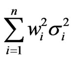
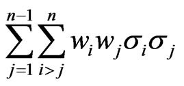
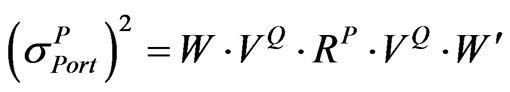
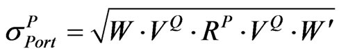
The objection of this section is to illustrate the method employed by CBOE [6] for calculating their implied correlation index. The method starts from calculating the variance of the portfolio . Given that the portfolio consists of n assets,
  can be calculated from Equation (1)
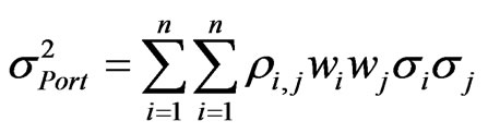 . (1)
. (1)
where:
 = Standard deviation or volatility of the portfolio (per annum).
 = Weight of asset i and j.
 = Standard deviation or volatility of asset i and j (per annum).
 = Correlation coefficient between asset i and j.
 .
.
If all correlation coefficients in the correlation matrix are assumed to be identical, then all  for i ≠ j is equal to r in which r is a constant real number lying within the closed interval [–1, 1]. The correlation matrix with such correlation coefficients is called equicorrelation matrix. Suppose that the equicorrelation matrix is being used to describe the relationship among assets in the portfolio, Equation (1) can be rewritten as:
 . (2)
. (2)
Thus, a closed-form formula of r can be derived by simple rearrangement of Equation (2).
 (3)
(3)
Since ,
,  , and
, and  are non-negative number, the terms
and
will also be non-negative number. For this reason, if , and
, and  remain unchanged, the higher
  will result in higher r; on contrary, the lower
  will result in lower r.
Further, the Equation (3) can also be used to calculate the implied correlation coefficient  of equicorrelation matrix by simply changing the volatility to be implied volatility as follows:
 . (4)
. (4)
where:
 = Implied volatility of the portfolio (per annum).
 = Implied volatility of asset i and j (per annum).
Although the CBOE implied correlation index assumes equicorrelation matrix, it is considered to be useful for hedging correlation risk or indicate overall correlation trend. However, because of unrealistic correlation assumption, equicorrelation matrix not be widely accepted for other applications, for instance, option pricing, portfolio allocation, or risk quantification.
3. Buss and Vilkov’s Method
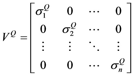
To the best of our knowledge, Buss and Vilkov’s method [4] is the only existing method for calculating realistic implied correlation matrix. So this section aims to give an overview of Buss and Vilkov’s method. The underlying concept of realistic of having realistic implied correlation is that every asset shouldn’t share the same correlation coefficient. For example, assets in the same industry should be more correlated together; assets with high market cap should be less correlated to assets with low market cap. Thus, it is important to have a prior knowledge about correlation matrix structure of portfolio that we want to extract realistic implied correlation matrix . Assume that
  is a valid correlation matrix under the objective measure, we are interested in obtaining a valid
  from
from  where the valid correlation matrix is defined in Definition 1.
Definition 1. An  valid correlation matrix must have the following characteristics:
1) Diagonal entries must be 1;
2) Non-diagonal entries are real numbers lying in the closed interval [–1, 1];
3) The correlation matrix is symmetric; and
4) The correlation matrix must be positive semi-definite.
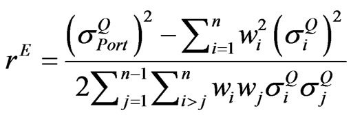
When correlation coefficients among assets are not identical, the implied volatility of the portfolio  can be described as:
 . (5)
. (5)
where:


or
 (6)
(6)
Because ,
,  , and
, and  are non-negative number, the terms
 and
and 
are also non-negative number. Given that other variables in Equation (6) are fixed, an increase in any of  will result in a rise in
 . Likewise, a decrease in any of
  will result in a drop in
 . To be realistic,
  must not be an equicorrelation matrix where all
  are identical, but
  should be a function of
 .
.
Buss and Vilkov [4] use the theory similar to the weighted average correlation matrices (WACM) method [7] to extract realistic correlation matrix in which the realistic correlation coefficient  is set to
 , where
 . Suppose that U is the square matrix with n dimensions with all elements are 1, the above assumption can be written in matrix form as:
 . (7)
. (7)
By substituting Equation (7) into Equation (5), it is straightforward to show that the following equation can be obtained:
 . (8)
. (8)
Once  is found, we can easily calculate
  from Equation (7).
Let  be the implied volatility of the portfolio obtained from
 , which can be described by Equation (9) or Equation (10):
 (9)
(9)
 (10)
(10)
Since every element in  is greater than or equal to zero,
  will be positive only when
 . However, positive may cause the realistic correlation matrix
  to be invalid when
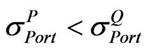 . That is the reason why, we propose another algorithm that can handle such cases.
4. New Algorithm for Obtaining Realistic Implied Correlation Matrix
According to WACM [7], suppose that and are valid correlation matrices with n dimensions. And the weight (w) is a real number in the closed interval [0,1]. If , then C must be a valid correlation matrix. Let U and L be the equicorrelation matrix of 1 and
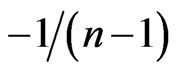 . Further, it is important to note that U and L are the valid upper bound and valid lower bound of equicorrelation matrix respectively.
Suppose that B and C are replaced by  and
and  accordingly, we will get:
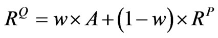 (11)
(11)
By simple formula rearrangement, we can obtain:
 (12)
(12)
By substituting Equation (12) into Equation (5), it is straightforward to show that the following equation can be obtained:
 (13)
(13)
The four-step algorithm for obtaining realistic implied correlation matrix from implied correlation index is then:
Step 1: Calculate the  by using Equation (10).
Step 2: Select the boundary matrix (U or L) based on relationship between two implied volatilities of portfolio ( and
and ).
).
• If , 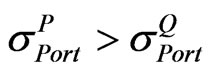 then we will set A = L.
The lower bound matrix (L) is selected. It means that we need to adjust  down toward L to obtain the realistic implied correlation matrix
 .
.
• If ,  then we will set A = U.
The upper bound matrix (U) is selected. It means that we need to adjust  up toward U to obtain the realistic implied correlation matrix
 .
.
Step 3: Compute w by using Equation (13) according to the choice of A in step 2.
• When , w can be calculated from:
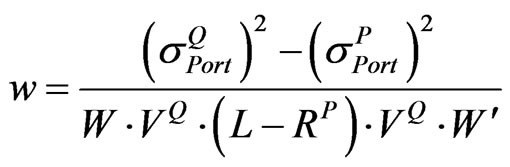 (14)
(14)
• When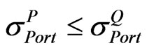 , w can be calculated from:
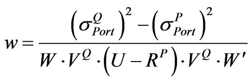 (15)
(15)
Step 4: Calculate the realistic implied correlation matrix  using Equation (12) based on w from the previous step.
5. Hypothetical Example
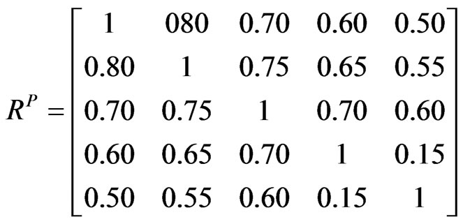
Suppose that we are interested to find a realistic implied correlation matrix of a hypothetical portfolio of five assets as described in Table 1.
Let the implied volatility of portfolio 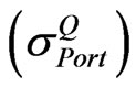 be 0.17. The following matrices are extracted from the information given in Table 1:
 (16)
(16)
 (17)
(17)
 (18)
(18)
The minimum eigenvalue of  is 0.1435. So it ensures that
  is a valid correlation matrix. Then, we can start using the above algorithm to obtain realistic implied correlation matrix
 .
.
In the first step, we use Equation (10) and information in Equations (16)-(18) to obtain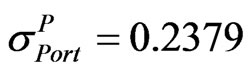 .
.
For this scenario, . So the matrix A is set to be equal to L in Equation (19) because
 .
.
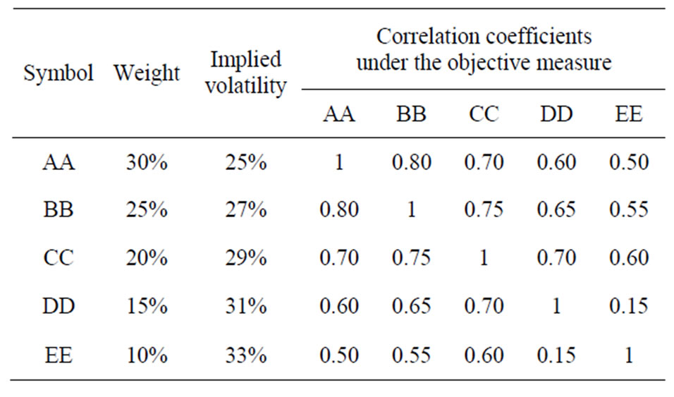
Table 1. The hypothetical portfolio of five assets.
 (19)
(19)
By using Equation (14), we can then obtain w = 0.5016. Finally, by substituting w into Equation (12),  will be:
 (20)
(20)
The above  is still a positive semi-definite as its minimum eigenvalue is 0.6882. By calculating
  from Equations (5), (16), (17), and (20). Then
  can be obtained. This proves that the Equation (20) is the correlation matrix that can make the portfolio volatility equal to implied volatility of the portfolio. Since
  in Equation (20) is generated based on
  and not an equicorrelation matrix, we can conclude that it’s a realistic implied correlation matrix. As a result, ones can use this correlation matrix in other application such as pricing basket options.
In comparison with the existing method introduced in Buss and Vilkov [4],  from Equation (8) is calculated. Based on the information in this example,
  , which is not in the range of (–1, 0]. In theory, the
  in Equation (21) that is generated from Equation (7) based on out-of-range
  may not be positive semi-definite.
 (21)
(21)
The minimum eigenvalue of  in Equation (21) is –0.0323. Although this
  can generate
 , this
  is not positive semi-definite nor valid anymore.
6. Results
In the above example, we compare the performance of our new algorithm (NA) and the existing method (BV) introduced by Buss and Vilkov [4]. The empirical example of the CBOE S&P 500 Implied Correlation Index (CSPICX) from CBOE [6] will be used throughout this section (see Table 2).

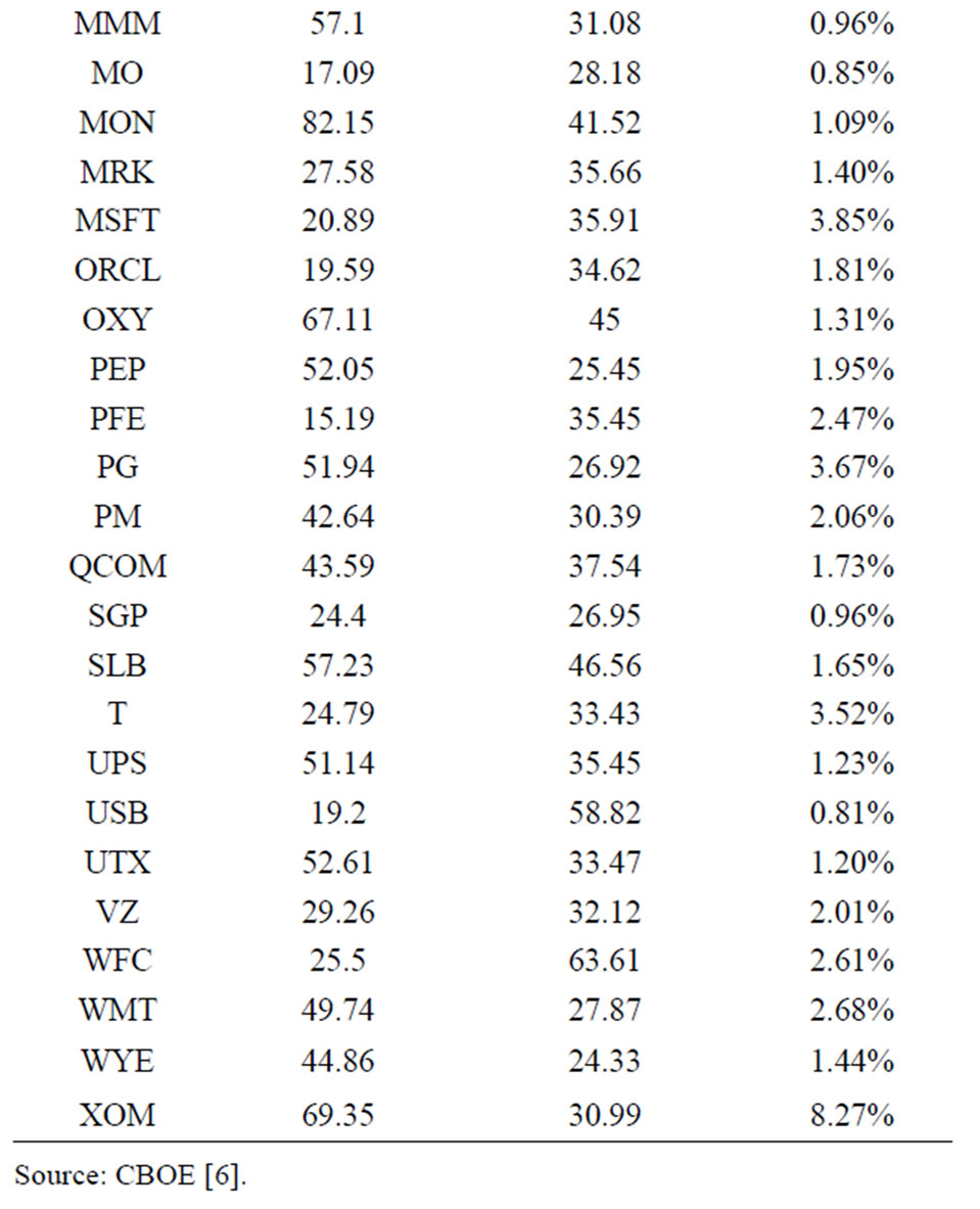
Table 2. Information of SPX stocks on May 29, 2009.
Theoretically, the CSPICX is the correlation coefficient of equicorrelation matrix, which can be derived by using Equation (4). However, for this index, not all underlying assets in the S&P500 index (SPX) are used in the calculation. Other than implied volatility of SPX options, we only need to use the information of 50 largest underlying assets in SPX and their options to calculate CSPICX. By assuming that the portfolio of SPX consisted of 50 underlying assets, the minimum and maximum values of its valid equicorrelation matrix is −1/49 and 1 respectively. Further, these boundaries can be applied to CSPICX because it is derived based on the assumption of equicorrelation matrix with 50 underlying assets.
To test the performance, we first assume that the CSPICX is lying in the open interval of (–1/49, 1) and the valid correlation matrix under the objective measure  is randomly generated by using the algorithm in [8]. Then we can calculate the following variables:
1) Implied volatility of the portfolio of SPX  by using Equation (2).
2)  and
and  based on Buss and Vilkov [4] by using Equations (8) and (7) respectively.
3) w and  based on the new algorithm introduced in the previous section by using Equations (13) and (12) respectively.
Based on our experiments of 1 million simulations, we cannot find any invalid . However, as shown in Figure 1, the probability of correlation matrix
  being invalid rises as CSPICX drops. This invalidity arises from the decrease of
 , which leads to the higher chance of having
 . Thus we can clearly see that NA can outperform BV for obtaining valid realistic correlation matrix in terms of stability of the solution.
7. Concluding Remarks
The proposed algorithm in this article allows us to obtain a realistic and valid implied correlation matrix given that a valid implied equicorrelation matrix can be obtained from the same set of information. In other words, the implied correlation index or the correlation coefficient of implied equicorrelation matrix must be in the closed interval , where n is the dimension of correlation matrix. It’s worth nothing that the method in Buss and Vilkov [4] can achieve the same objective, but the scope is more limited. This new algorithm outperforms both Buss and Vilkov’s and CBOE methods because it can be used to obtain a valid implied correlation matrix. Once the realistic and valid implied correlation matrix can be obtained, we can use this information in various applications, such as portfolio optimization, stress testing, option pricing, dispersion trading, and so forth.