Continuous Iteratively Reweighted Least Squares Algorithm for Solving Linear Models by Convex Relaxation

Abstract

In this paper, we present continuous iteratively reweighted least squares algorithm (CIRLS) for solving the linear models problem by convex relaxation, and prove the convergence of this algorithm. Under some conditions, we give an error bound for the algorithm. In addition, the numerical result shows the efficiency of the algorithm.

Share and Cite:

Luo, X. and Ye, W. (2019) Continuous Iteratively Reweighted Least Squares Algorithm for Solving Linear Models by Convex Relaxation. Advances in Pure Mathematics, 9, 523-533. doi: 10.4236/apm.2019.96024.

1. Introduction

Low-dimensional linear models have broad applications in data analysis problems such as computer vision, pattern recognition, machine learning, and so on [1] [2] [3] . In most of these applications, the data set is noisy and contains numbers of outliers so that they are distributed in higher dimensional. Meanwhile, principal component analysis is the standard method [4] for finding a low-dimensional linear model. Mathematically, the problem can be present as

min x χ x Π x 2 subject to Π is an orthoprojector and t r Π = d (1)

where χ is the data set consisting of N points in D , x D , a target dimension d { 1,2, , D 1 } , 2 denotes the l 2 norm on vectors, and tr refers to the trace.

Unfortunately, if the data set contains a large number of noise in the inliers and a substantial number of outliers, these nonidealities points can interfere with the linear models. To guard the subspace estimation procedure against outliers, statistics have proposed to replace the l 2 norm [5] [6] [7] with l 1 norm that is less sensitive to outliers. This idea leads the following optimization problem

min x χ x Π x subject to Π is an orthoprojector and t r Π = d (2)

The optimization problem (2) is not convex, and we have no right to expect that the problem is tractable [8] [9] . Wright [10] proved that most matrices can be efficiently and exactly recovered from most error sign-and-support patterns by solving a simple convex program, for which they give a fast and provably convergent algorithm. Later, Candes [11] presented that under some suitable assumptions, it is possible to recover the subspace by solving a very convenient convex program called Principal Component Pursuit. Base on convex optimization, Lerman [12] proposed to use a relaxation of the set of orthogonal projectors to reach the convex formulation, and give the linear model as follows

min x χ x P x subjectto 0 P I and t r P = d (3)

where the matrix P is the relaxation of orthoprojector Π , whose eigenvalues lie in the interval [ 0,1 ] form a convex set. The curly inequality denotes the semidefinite order: for symmetric matrices A and B, we write A B if and only if B A is positive semidefinite, the problem (3) is called REAPER.

To obtain a d-dimensional linear model from a minimizer of REAPER, we need to consider the auxiliary problem

min x χ P Π S 1 subjectto Π is an orthoprojector and t r Π = d (4)

where P is an optimal point of REAPER, S 1 denotes Schatten 1-norm, in other words, the orthoprojector Π is closest to P in the Schatten 1-norm, and the range of Π is the linear model we want. Fortunately, Lerman has given the error bound between the d-dimensional subspace with the d-dimensional orthoprojector Π in Theorem 2.1 [12] .

In this paper, we improve that the algorithm calls continuous iteratively reweighted least squares algorithm for solving REAPER (3), and under a weaker assumption on the data set, we can prove the algorithm is convergent. In the experiment part, we compare the algorithm with the IRLS algorithm [12] .

The rest of the paper is organized as follows. In Section 2, we develop the CIRLS algorithm for solving problem (3). We present a detail convergence analysis for the CIRLS algorithm in Section 3. An efficient numerical is reported in Section 4. Finally, we conclude this paper in Section 5.

2. The CIRLS Algorithm

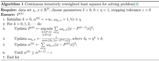
We give the CIRLS algorithm for solving optimization problem (3), and the algorithm is summarized as Algorithm 1.

In the next section, we prove the sequence { P ( k ) } k 1 is convergent to P δ . Furthermore, we also present the P δ satisfied the bound with the optimal point P of REAPER.

3. Convergence of CIRLS Algorithm

In this section, we prove that the sequence { P ( k ) } k 1 generated by Algorithm 1 is convergent to P δ and we provide the P δ satisfied the bound with the optimal point P of REAPER. Firstly, we start from the Lemma prepare for the proof of the following theorem.

Lemma 1 ( [12] , Theorem 4.1) Assume that the set χ of observations does not lie in the union of two strict subspaces of D . Then the iterates of IRLS Algorithm with ε = 0 converge to a point P δ that satisfies the constraints of the REAPER problem. Moreover, the objective value at P δ satisfies the bound

x χ x P δ x x χ x P x 1 2 δ | χ | , (5)

where P is an optimal point of REAPER.

In lemma 1, under the assumption that the set χ of observations does not lie in the union of two strict subspaces of D , they consider the convergence of the IRLS algorithm. However, verify whether a data set satisfies this assumption requires amounts of computation in theory, so we give a assumption that is easier to verify in following theorem.

Theorem 1 Assume that the set χ of observations satisfies s p a n { χ } = D , if P δ is the limit point of the sequence { P ( k ) } k 1 generated by C I R L S δ algorithm, then P δ is an optimal point of the following optimization problem

min ( { x : x P x δ } x P x + 1 2 { x : x P x < δ } { x P x 2 δ + δ } ) subjectto 0 P I and t r P = d , (6)

and satisfies

x χ x P δ x x χ x P x 1 2 δ | χ | , (7)

where P is an optimal point of REAPER(3).

Proof. Firstly, we consider the optimization model with Algoritnm 1,

min ( { x : x P x δ } x P x + 1 2 { x : x P x < δ } { x P x 2 δ + δ } ) subjectto 0 P I and t r P = d , (8)

then, we define iterative point P ( k + 1 ) of the optimization problem

P ( k + 1 ) : = arg min x χ ω δ k , x x P x 2 subjectto 0 P I and t r P = d . (9)

where ω δ k , x : = 1 max { δ k , x P ( k ) x } .

For convenience, let Q = I P , and the optimization model(9) convert into

Q ( k + 1 ) : = arg min 0 Q I t r Q = D d x χ ω δ k , x Q x 2 . (10)

where ω δ k , x : = 1 max { δ k , Q ( k ) x } .

Similarly, we convert the optimization model (8) into

min F δ ( Q ) = min ( { x : Q x δ } Q x + 1 2 { x : Q x < δ } ( Q x 2 δ + δ ) ) subjectto 0 Q I and t r Q = D d . (11)

Next we prove the convergence of P ( k ) , consider the Huber-like function

H δ k ( x , y ) = { 1 2 ( x 2 δ k + δ k ) 0 y < δ k 1 2 ( x 2 y + y ) y δ k (12)

since 1 2 ( x 2 y + y ) | x | , for any y > 0 , then

H δ k ( x , y ) H δ k ( x , | x | ) . (13)

holds for any y > 0 , x R . We introduce the convex function

F δ k ( Q ) : = x χ H δ k ( Q x , Q x ) = { x χ : Q x δ k } Q x + 1 2 { x χ : Q x < δ k } ( Q x 2 δ k + δ k ) , (14)

note that F is continuously differentiable at each matrix Q, and the gradient is

F δ k ( Q ) = { x χ : Q x δ k } Q x x T Q x + { x χ : Q x < δ k } Q x x T δ k = x χ Q x x T max { δ k , Q x } . (15)

in addition, we introduce the function

G δ k ( Q , Q ( k ) ) : = x χ H δ k ( Q x , Q ( k ) x ) = { x χ : Q ( k ) x δ k } 1 2 ( Q x 2 Q ( k ) x + Q ( k ) x ) + { x χ : Q ( k ) x < δ k } 1 2 ( Q x 2 δ k + δ k ) , (16)

then

G δ k ( Q , Q ( k ) ) = x χ Q x x T max { δ k , Q ( k ) x } . (17)

By the definition of G δ k ( Q , Q ( k ) ) we know that

G δ k ( Q ( k ) , Q ( k ) ) = x χ H δ k ( Q ( k ) x , Q ( k ) x ) = F δ k ( Q ( k ) ) , (18)

and

G δ k ( Q ( k ) , Q ( k ) ) = x χ Q ( k ) x x T max { δ k , Q ( k ) x } = F δ k ( Q ( k ) ) , (19)

it is obvious that G δ k ( , Q ( k ) ) is a smooth quadratic function, we may relate G δ k ( , Q ( k ) ) through the expansion in Q ( k ) as follows

G δ k ( Q , Q ( k ) ) = F δ k ( Q ( k ) ) + Q Q ( k ) , F δ k ( Q ( k ) ) + 1 2 Q Q ( k ) , C k ( Q ( k ) ) ( Q Q ( k ) ) , (20)

where C k ( Q ( k ) ) = x χ x x T max { δ k , Q ( k ) x } is the Hessian matrix of G δ k ( Q , Q ( k ) ) .

By the definition of G δ k ( Q , Q ( k ) ) we know that F δ k ( Q ) = G δ k ( Q , Q ) , combines with (13) we have

F δ k ( Q ) = x χ H δ k ( Q x , Q x ) x χ H δ k ( Q x , Q ( k ) x ) = G δ k ( Q , Q ( k ) ) , (21)

and since the optimization model(10) is equivalent to the model

Q ( k + 1 ) : = arg min 0 Q I t r P = D d G δ k ( Q , Q ( k ) ) , (22)

then we have the monotonicity property

F δ k ( Q ( k + 1 ) ) G δ k ( Q ( k + 1 ) , Q ( k ) ) G δ k ( Q ( k ) , Q ( k ) ) = F δ k ( Q ( k ) ) . (23)

We note that when x 0 , we have

H δ k ( x , x ) = { x x δ k 1 2 ( x 2 δ k + δ k ) 0 x < δ k (24)

H δ k + 1 ( x , x ) = { x x δ k + 1 1 2 ( x 2 δ k + 1 + δ k + 1 ) 0 x < δ k + 1 (25)

since δ k + 1 < δ k , on the one hand, when x δ k + 1 , H δ k + 1 ( x , x ) = x holds, and H δ k ( x , x ) x holds for any x R , therefore the inequality H δ k + 1 ( x , x ) H δ k ( x , x ) holds for x δ k + 1 . On the other hand, when x < δ k + 1 ,

H δ k + 1 ( x , x ) = 1 2 ( x 2 δ k + 1 + δ k + 1 ) , and H δ k ( x , x ) = 1 2 ( x 2 δ k + δ k ) holds, then we have

H δ k ( x , x ) H δ k + 1 ( x , x ) = 1 2 ( x 2 δ k x 2 δ k + 1 + δ k δ k + 1 ) = 1 2 ( δ k δ k + 1 ) ( 1 x 2 δ k δ k + 1 ) . (26)

since δ k > δ k + 1 , and x < δ k + 1 , H δ k ( x , x ) H δ k + 1 ( x , x ) > 0 holds for all x 0 , therefore

F δ k + 1 ( Q ( k + 1 ) ) = x χ H δ k + 1 ( Q ( k + 1 ) x , Q ( k + 1 ) x ) x χ H δ k ( Q ( k + 1 ) x , Q ( k + 1 ) x ) = F δ k ( Q ( k + 1 ) ) , (27)

and according to (23), we have the following result

F δ k + 1 ( Q ( k + 1 ) ) F δ k ( Q ( k ) ) . (28)

Since

Q ( k + 1 ) = arg min 0 Q I t r Q = D d G δ k ( Q , Q ( k ) ) , (29)

combined with the convex optimization variational inequalities with some constraints, we have

0 Q Q ( k + 1 ) , G δ k ( Q ( k + 1 ) , Q ( k ) ) 0 Q I , t r Q = D d , (30)

base on (20), we have the equation

G δ k ( Q , Q ( k ) ) = F δ k ( Q ( k ) ) + C k ( Q ( k ) ) ( Q Q ( k ) ) , (31)

then we have

0 Q ( k ) Q ( k + 1 ) , F δ k ( Q ( k ) ) + C k ( Q ( k ) ) ( Q ( k + 1 ) Q ( k ) ) , (32)

therefore

G δ k ( Q ( k + 1 ) , Q ( k ) ) = F δ k ( Q ( k ) ) + Q ( k + 1 ) Q ( k ) , F δ k ( Q ( k ) ) + 1 2 Q ( k + 1 ) Q ( k ) , C k ( Q ( k ) ) ( Q ( k + 1 ) Q ( k ) ) F δ k ( Q ( k ) ) Q ( k + 1 ) Q ( k ) , C k ( Q ( k ) ) ( Q ( k + 1 ) Q ( k ) )

+ 1 2 Q ( k + 1 ) Q ( k ) , C δ k ( Q ( k ) ) ( Q ( k + 1 ) Q ( k ) ) F δ k ( Q ( k ) ) 1 2 Q ( k + 1 ) Q ( k ) , C k ( Q ( k ) ) ( Q ( k + 1 ) Q ( k ) ) , (33)

and according to(23), then we get the inequality

F δ k ( Q ( k + 1 ) ) F δ k ( Q ( k ) ) 1 2 Q ( k + 1 ) Q ( k ) , C k ( Q ( k ) ) ( Q ( k + 1 ) Q ( k ) ) , (34)

add to F δ k + 1 ( Q ( k + 1 ) ) F δ k ( Q ( k + 1 ) ) , then we have

1 2 Q ( k + 1 ) Q ( k ) , C δ k ( Q ( k ) ) ( Q ( k + 1 ) Q ( k ) ) F δ k ( Q ( k ) ) F δ k + 1 ( Q ( k + 1 ) ) . (35)

Let m : = max k 1 { δ k , max x χ { x } } , since Q ( k + 1 ) , Q ( k ) and C k ( Q ( k ) ) are all symmetric matrix, then the inequality

Q ( k + 1 ) Q ( k ) , C k ( Q ( k ) ) ( Q ( k + 1 ) Q ( k ) ) t r ( ( Q ( k + 1 ) Q ( k ) ) 2 C k ( Q ( k ) ) ) , (36)

holds, in addition, 0 Q ( k + 1 ) I , 0 Q ( k ) I , thus ( Q ( k + 1 ) Q ( k ) ) 2 is positive semidefinite matrix, and Q ( k ) x Q ( k ) x x , then we have max { δ k , Q ( k ) x } max { δ k , x } m , therefore

C k ( Q ( k ) ) = x χ x x T max { δ k , Q ( k ) x } 1 m x χ x x T 1 m λ min ( x χ x x T ) I , (37)

so we have

( Q ( k + 1 ) Q ( k ) ) 2 C k ( Q ( k ) ) 1 m λ min ( x χ x x T ) ( Q ( k + 1 ) Q ( k ) ) 2 , (38)

thus we can get the inequality as follows

t r ( Q ( k + 1 ) Q ( k ) ) 2 C k ( Q ( k ) ) 1 m λ min ( x χ x x T ) Q ( k + 1 ) Q ( k ) F 2 . (39)

Let μ = 1 2 m λ min ( x χ x x T ) , then μ > 0 , and we have

Q ( k + 1 ) Q ( k ) F 2 1 μ ( F δ k ( Q ( k ) ) F δ k + 1 ( Q ( k + 1 ) ) ) , (40)

since F δ k ( Q ) 0 , so we have

k = 1 Q ( k + 1 ) Q ( k ) F 2 1 μ F δ 1 ( Q ( 1 ) ) < + , (41)

therefore, we get the following limits

lim k Q ( k + 1 ) Q ( k ) F = 0. (42)

Since the set { Q : 0 Q I , t r Q = D d } is bounded and closed convex set, and Q ( k + 1 ) { Q : 0 Q I , t r Q = D d , k = 1,2, } , then the sequence { Q ( k ) } k 1 exist convergent subsequences, we suppose { Q ( k i ) } i 1 is one of the subsequences and

Q ˜ = lim i + { Q ( k i ) } . (43)

Since for any i 1 , we have

Q ( k i + 1 ) Q ˜ F = Q ( k i + 1 ) Q ( k i ) + Q ( k i ) Q ˜ F Q ( k i + 1 ) Q ( k i ) F + Q ( k i ) Q ˜ F , (44)

and

lim k Q ( k + 1 ) Q ( k ) F = 0 , (45)

so we have

lim i + Q ( k i + 1 ) Q ˜ F = 0 , (46)

in other words

lim i + Q ( k i + 1 ) = Q ˜ . (47)

According to the definition of Q ( k i + 1 ) and (10), for any Q : 0 Q I , t r Q = D d , we have

0 Q Q ( k i + 1 ) , F δ k i ( Q ( k i ) ) + C k i ( Q ( k i ) ) ( Q ( k i + 1 ) Q ( k i ) ) . (48)

Since

lim i + F δ k i ( Q ( k i ) ) = lim i + x χ Q ( k i ) x x T max { δ k i , Q ( k i ) x } = x χ lim i + Q ( k i ) x x T max { δ k i , Q ( k i ) x } = x χ Q ˜ x x T max { δ , Q ˜ x } = F δ ( Q ˜ ) (49)

and

C k i ( Q ( k i ) ) ( Q ( k i + 1 ) Q ( k i ) ) F = x χ x x T max { δ k i , Q ( k i ) x } ( Q ( k i + 1 ) Q ( k i ) ) F x χ x x T F max { δ k i , Q ( k i ) x } Q ( k i + 1 ) Q ( k i ) F ( x χ x x T F δ k i ) Q ( k i + 1 ) Q ( k i ) F 1 δ ( x χ x x T F ) Q ( k i + 1 ) Q ( k i ) F (50)

as well as Q ( k i + 1 ) Q ( k i ) F 0 ( i + ) , so we have

lim i + C k i ( Q ( k i ) ) ( Q ( k i + 1 ) Q ( k i ) ) F = 0 , (51)

thus

lim i + C k i ( Q ( k i ) ) ( Q ( k i + 1 ) Q ( k i ) ) = 0. (52)

Taking the limit at both ends of the inequality (48) and using the continuity of the inner product, for any Q : 0 Q I , t r Q = D d , we have

0 Q Q ˜ , F δ ( Q ˜ ) , (53)

the variational inequalities demonstrate that

Q ˜ = arg min F δ ( Q ) subjectto 0 Q I , t r Q = D d , (54)

it means that the limit points Q δ of any convergent subsequence generated by { Q ( k ) } k 1 is an optimal point of the following optimization problem

Q δ = arg min F δ ( Q ) subjectto 0 Q I , t r Q = D d . (55)

Now we set P δ = I Q δ and define F 0 ( P ) : = x χ ( I P ) x with 0 P I and t r P = d . And we define F δ ( P ) : = x χ H δ ( ( I P ) x , ( I P ) x ) , and P : = arg min F 0 ( P ) with respect to the feasible set 0 P I , and t r P = d , then we have

P δ = arg min F δ ( P ) , subjectto 0 P I , t r Q = d . (56)

According to the lemma 3.1, we have

0 F 0 ( P δ ) F 0 ( P ) 1 2 δ | χ | , (57)

where | χ | denotes the number of elements of χ .

4. Numerical Experiments

In this section, we present a numerical experiment to show the efficiency of the CIRLS algorithm for solving problem (3). We compare the performance of our algorithm with IRLS on the data generated from the following model. In the test, we randomly choose Nin inliers sampled from the d-dimensional Multivariate Normal distribution N ( 0, Π L ) on subspace L and add Nout outliers sampled from a uniform distribution on [ 0,1 ] D , we also add a Gaussian noise N ( 0, ε 2 I ) . The experiment is performed in R and all the experimental results were averaged over 10 independent trials.

The parameters were set the same as [12] that ε = 10 15 , ε = 0.01 and

δ = 10 10 , we choose η from [ 0,1 ] and we set η = 1 2 in general. All the

other parameters of the two algorithms were set to be the same, Nout means the number of outliers and Nin is the number of inliers, D is the ambient dimension and d is the subspace dimension we want. From the model above, we get the data sets with values in the table below, then we calculate the iterative number

Table 1. The iterative number of the CIRLS and IRLS for different dimension.

n ( iterative ) with the two algorithms through the data sets and the given parameters. The results are shown in Table 1.

We focus on the convergence speed of the two algorithms. Table 1 reports the numerical results of the two algorithms for different space dimension. From the result, we can see that in different dimension, the CIRLS algorithm performs better than IRLS algorithm in convergent efficiency.

5. Conclusion

In this paper, we propose an efficient continuous iteratively reweighted least squares algorithm for solving REAPER problem, and we prove the convergence of the algorithm. In addition, we present a bound between the convergent limit and the optimal point of REAPER problem. Moreover, in the experiment part, we compare the algorithm with the IRLS algorithm to show that our algorithm is convergent and performs better than IRLS algorithm in the rate of convergence.

Conflicts of Interest

The authors declare no conflicts of interest regarding the publication of this paper.

References

[1] Torre, F.D. and Black, M.J. (2001) Robust Principal Component Analysis for Computer Vision. Proceedings of Eighth IEEE International Conference on Computer Vision, Vancouver, 7-14 July 2001, 362-369.
https://doi.org/10.1109/ICCV.2001.937541
[2] Wanger, A., Wright, J. and Ganesh, A. (2009) Towards a Practical Face Recongnition System: Robust Registration Tillumination by Sparse Represention. 2009 IEEE Conference on Computer Vision and Pattern Recognition, Miami, FL, 20-25 June 2009, 20-25.
https://doi.org/10.1109/CVPR.2009.5206654
[3] Ho, J., Yang, M., Lim, J., Lee, K. and Kriegman, D. (2003) Clustering Appearances of Objects under Varying Illumination Conditions. 2003 IEEE Computer Vision and Pattern Recognition, Madison, WI, 18-20 June 2003, 11-18.
[4] Jolliffe, I.T. (2002) Principal Component Analysis. Journal of Marketing Research, 25, 513.
[5] Watson, G.A. (2002) On the Gauss-Newton Method for l1 Orthogonal Distance Regression. IMA Journal of Numerical Analysis, 22, 345-357.
https://doi.org/10.1093/imanum/22.3.345
[6] Ding, C., Zhou, D., He, X. and Zha, H. (2006) R1-PCA: Rotational Invariant L1-Norm Principal Component Analysis for Robust Subspace Factorization. The 23rd International Conference on Machine Learning, 23, 281-288.
https://doi.org/10.1145/1143844.1143880
[7] Kwak, N. (2008) Principal Component Analysis Based on L1-Norm Maximization. IEEE Transactions on Pattern Analysis and Machine Intelligence, Pittsburgh, PA, 25-29 June 2006, 1672-1680.
https://doi.org/10.1109/TPAMI.2008.114
[8] Maronna, R.A., Martin, D.R. and Yohai, V.J. (2006) Robust Statistics. Wiley Series in Probability and Statistics. Wiley, Chichester.
https://doi.org/10.1002/0470010940
[9] Zhang, T., Szlam, A. and Lerman, G. (2009) Median K-Flats for Hybrid Linear Modeling with Many Outliers. IEEE International Conference on Computer Vision Workshops, 12, 234-241.
[10] Wright, J., Peng, Y.G. and Ma, Y. (2009) Robust Principal Component Analysis: Exact Recovery of Corrupted Low-Rank Matrices by Convex Optimization. 2009 23rd Annual Conference on Neural Information Processing Systems, Vancouver, Canada, 7-10 December 2009, 2080-2088.
[11] Candes, E.J., Li, X., Ma, Y. and Wright, J. (2011) Robust Principal Component Analysis? Journal of the ACM, 58, Article No. 11.
https://doi.org/10.1145/1970392.1970395
[12] Lerman, G., McCoy, M.B., Tropp, J.T. and Zhang, T. (2015) Robust Computation of Linear Models by Convex Relaxation. Foundations of Computational Mathematics, 15, 363-410.
https://doi.org/10.1007/s10208-014-9221-0

Copyright © 2024 by authors and Scientific Research Publishing Inc.

Creative Commons License

This work and the related PDF file are licensed under a Creative Commons Attribution 4.0 International License.