A Model of the Market Process with Numerical Simulation

Ricardo Luis Chaves Feijó, Fabio Barbieri

School of Economics, Business Administration and Accounting at Ribeirao Preto, University of Sao Paulo, Sao Paulo, Brazil.

DOI: 10.4236/me.2018.911118                

Abstract

The paper simulates the price-arbitrage process at the market for homogeneous good and tries to show the convergence into a single price from different cross-linked markets of this homogeneous good. It examines the problem by random generation of values in the simulation environment offered by the Matlab program. It is emphasized here the approach in which the agent’s alertness is crucial to the market. The emphasis is not on the price that equilibrates supply and demand, since there is not a single price for a homogeneous commodity. A homogeneous good is negotiated with different prices in different parts of a market. The paper explains the process in which the agent’s alertness leads to a uniform price in terms of a simulation model, in the belief that that technique leads to a better understanding of the precise nature of the market process and the agent’s alertness role in equilibration. The paper also discusses the effects of the heterogeneous agents and market barriers in the market convergence process. The innovative feature of the paper is the simulation experiment.

Keywords

Numerical Simulation, Alertness, Market Process

1. Introduction

Two main pointes make us believe that the paper has the potential to contribute to the literature. First, numerical simulations seem to be a fruitful way to study market process and price convergence, in particular. Second, the inclusion of alertness itself as a determinant of the probability of discovery of new markets is an interesting and novel assumption.

Forty-eight years ago, Littlechild and Owen [1] developed an algebraic model to describe the market process. They claimed to be the mathematical formalization of the Austrian school’s view of the market process. However, such a model distorts the fundamental meaning of the Austrian dynamics approach on market. It does not faithfully follow Ludwig von Mises’s approach to the market process, it is not faithful to the concept of equilibrium of this school (logical equilibrium and not mathematical one), it does not describe the price mechanism as Austrian economists do, does not effectively address the role of the entrepreneurial activity on the functioning of the markets.1 In short, though pioneering, it had been a failed attempt to give Austrian insights a mathematical treatment.2

Nevertheless, the structure of the model developed in the pioneer paper allows an interesting computational approach to the process of price arbitrage in the markets for a homogeneous good. In particular, it is important to show the possibility of converging to a single price for the good in question when the markets are initially isolated from one another and are gradually linked by the agents’ own arbitration process, as they discover these markets and those are integrated with each other.

The idea that arbitrage would bring about a single price for homogeneous good is very old in economic thought.3 The intuition, widely disseminated in the profession, is that the quotations of homogeneous goods converge quickly at a single price by the agents’ action in the market. However, in the last century the scientific community has more technically examined the problem of uniform price formation in the markets and concluded that the process would not be so simple and immediate. In fact, a gigantic literature on learning (in particular prices) is accumulating, including decision errors and limited rationality. In addition, the growing treatment of the problem by computational methods and numerical simulation procedures is noted.4

In this spirit, we propose an interesting and original treatment of the basic problem of simultaneous price convergence of a homogeneous good practiced in different markets by means of random generation of values of the variables in the simulation environment offered by the Matlab program.5 The hypotheses of the new treatment are simple and follow in general the model of Littlechild and Owen, although with no pretense of being an Austrian representation of the market process. The point of advancement in relation to the pioneer model is the possibility of a probabilistic treatment of the process of discovery of new markets, or of new prices, through computational simulation exercises. Purely algebraic treatment and the corresponding price convergence theorems in different markets for a homogeneous good are not successful in incorporating into the equations the process of market discovery itself and their integration through arbitrage. In fact, such a process is only presupposed, and not demonstrated or evaluated as to its effectiveness; the speed of integration given the mechanism of discovery etc. The use of simulation, instead of mathematical analysis, allows a detailed study, though artificial data, of the dynamics of convergence taking into account the discoveries by the agents of new prices.

It is, therefore, a study on the role of knowledge and discovery in the process of price convergence in the markets; a relevant study even if, over time, the single convergence price is not necessarily the intertemporal equilibrium price. The single price obtained by the arbitrage of the markets, accompanied by increasing discoveries by the agents, would not be a final state for the price practiced in the linked markets (effectively arbitrated by a common set of agents). The study of uniform price formation, however, facilitates the investigation of the equilibrium price by allowing a single price to be assigned subsequently to each homogeneous good. In this setting, one can study the possibility that the traditional conditions of general equilibrium be met.

The central contribution of the essay lies in the use of computational simulations to model the discovery of new markets through a probabilistic process that controls the agent’s chance to discover a market, starting from its base, the place where he previously knows and arbitrates, by a distribution of probabilities whose variance depends on a particular propensity of the agent in question, his alertness.6

Although there is an enormous amount of studies dealing with the process of convergence of markets by discovery of new prices, we did not find any numerical simulation study with the use of a simple Matlab program and able to study the effectiveness of the convergence process and its sensitivity to the basic parameters of the model. When the problem of incomplete information in which economic agents operate is recognized, the traditional approach focuses more on the restrictive role of imperfect information and the costs of obtaining information. The genuinely Austrian approach incorporates a radical ignorance of the agents, which is not quantifiable, which is unknown to the analyst, and therefore very difficult to model. More than just assuming that agents are unaware of information sets, Austrians are concerned with studying the process by which information is revealed to agents and how they learning to interpret it. From this point of view, the discovery of information involves surprise and could not be priced. Economists at the Austrian school investigate to what extent and under what conditions such a discovery would lead the market toward equilibrium. In the real and complex economy, they ask whether there is a tendency to approach, rather than distancing, the equilibrium trajectory.

The proposed simulation model sheds new light on the process in which equilibrium is reached, with reference to a formal model that follows many aspects of pioneering treatment, however, with no pretense of formalizing the richness of the Austrian approach. It is only a model of numerical simulation of the process of convergence of prices in the markets. The emphasis is only on the arbitration process. At every moment, the price adjustment in each market obeys the law of supply and demand, and the interest is only in how different prices converge with the gradual integration of the markets by the agents’ arbitrage. Therefore, the emphasis of the study falls not on the concept of equilibrium itself, but on the mechanism of equilibration. A homogeneous good is transacted at different prices in different parts of a market because the market participant does not know all of it (knows only parts of it or submarkets). It is imagined here that, with the discovery of the agents, given the alertness of each one, a uniform price is arrived at. Given the price differences between the new market and the known markets, transfers of goods take place immediately. There is no lag between buying and selling in the model, within which prices could change. This price can, after being reached, be examined regarding its dynamic stability by a general equilibrium model, which does not belong to the scope of this study. It is then a question of providing a description of the process of price convergence in terms of a simulation exercise based on a mathematical model similar to that of Littlechild and Owen, but introducing an explicit and detailed hypothesis about the process of discovering new markets, treatable only through computer simulations, not mathematical analysis. It is believed that the present simulation exercise leads to a better understanding of the nature of price convergence in the markets and the role of agent discovery in this process.

In this sense, consideration is given to obtaining homogeneous prices for the performance of the computational model by drawing random variables when running the program in Matlab and obtaining artificial data. The paper also examines the speed of the convergence process, and how long it lasts, which depends on arbitrary parameters. At the end, some analysis of parameter variation is done and entry barriers are added. To do so, the paper is structured into five sections, in addition to this introduction. Section 2 presents the algebraic reference model in a synthetic way. Section 3 shows the extensions of the basic model and explains the numerical simulation technique. Section 4 presents the numerical simulation results for different sets of parameters. The penultimate section discusses the effects of the hypothesis of heterogeneous agents and market barriers in the process of market convergence before the brief concluding section of the essay.

2. Basic Structure of the Convergence

Here are seven basic hypotheses of the model:

1) It is assumed that a homogeneous commodity is transacted in a given set of markets (each segment is called a “submarket”) over a period. The homogeneous commodity hypothesis is just to simplify the model. By submarkets are meant isolated markets from other markets, in the sense that agents acting on it do not act on others.

2) Agents are price takers. That is, it is a model of perfect competition, or almost perfect, because the information is not complete.

3) The excess demand curves that form in each segment of the submarket are constant over time and are linear in relation to prices. The way prices respond to such excesses is always the same, given by a simple linear equation.

4) There is a single price in each submarket at every instant of time, which is determined only by the net quantity of commodities offered on it. Although prices vary with time, each time it is unique to each submarket.

5) The products are transferred between submarkets by the arbitrators. Each agent knows the existence of only a single set of submarkets. That is, it is an imperfect knowledge model in which learning involves research on the part of the agent.

6) Two processes occur simultaneously: arbitrage among known submarkets and new submarkets are known. At the same time, agents arbitrate submarkets and are alert to the discovery of new submarkets.

7) For each agent, the increase in the amount he transfers between submarkets is directly proportional to the price differences between two submarkets he arbitrates. The transfer rate, regulated by a constant of proportionality, varies according to the agent and denotes different impatience, precaution, flexibility and cost of adjustment. The constant is fixed per agent, and does not vary from one submarket to another.

The model does not consider production. There is a prevailing starting price in each submarket and, from this, price movements occur through the arbitrage action. In the supply, goods are transferred from the submarkets that practice lower prices to those with higher prices. Individual demand also responds to prices. The difference between these two forces generates, at each instant, an excess supply or net supply of goods by all agents in each submarket, which depends on the agents’ responses to price differences between them (transfer rates). In each sub-market, the supply varies with the price differences formed at each moment, considering the transfer rates, and a predetermined total amount of transacted goods is assumed so that the sum of the net offers is null, for all sub-markets.

In the original model of Littlechild and Owen, the probability of the agent discovering a new submarket is given by a constant invariant in time that reflects differences in the individual alertness. It is assumed that this probability is proportional to the price difference between the prices practiced in potentially arbitrated submarkets and relevant prices in the price range among previously known submarkets, but the constant of proportionality is greater the higher the alertness of the agent. In the simulation model of this essay, the alertness level of the agent is otherwise: it has a probability distribution governed by a normal curve, in which the variance depends on the degree of alertness of the agent in question.7 Drawings are made by the computer obeying the specified distribution that allows identifying the submarkets reached (and linked), as will be detailed later.8

It works with the hypothesis of division, such that different agents know different markets. At first, each agent knows only the price in their original market, not in all the markets in which they could operate. The discovery of prices involves some kind of cost, at least an expenditure with displacement. The agent must go to different sales stations (submarkets) and investigate the prices, for the same homogeneous good, practiced in these places. The greater the alertness, the greater the range of searched places. Hopefully, in some of them arbitrage possibilities will arise, which will be explored.

The model investigates theoretically how the arbitration process leads to a uniform price. To do this, it begins by defining two concepts:

1) Two directly linked submarkets occur when at least one agent knows both.

2) In indirectly linked submarkets, there is an intermediate chain of submarkets, which starts and ends in two of them, and each point of the chain is directly linked to the next.

Working with the same assumptions and concepts, but without detailing the discovery process, Littlechild and Owen [1] demonstrate mathematically that if two submarkets are linked (directly or indirectly) all prices will tend to converge at a uniform equilibrium price. The series of discoveries will lead to a link of all submarkets or to non-linked submarkets, whose prices will equal the uniform equilibrium price among the linked submarkets. A submarket may remain unknown to an agent if its prices converge quickly on the prices in submarkets already discovered, thereby reducing its chance of being discovered, even if it maintains a degree of attraction. The proof of these authors is purely mathematical, in the form of theorems.

The submarket set is represented by $M=\left\{1,2,\cdots ,m\right\}$ and the set of traders by $N=\left\{1,2,\cdots ,n\right\}$ . Trader j knows the existence of a fixed subset of submarkets $M_j\subseteq M$ . He can arbitrate in any submarket k such that $k\in M_j$ . $M_j$ can change with time. If the submarkets k and $k^{\prime }$ are such that $k,k^{\prime }\in M_j$ , they are directly linked. They are indirectly linked if there is a submarket chain $k_0,k_1,\cdots ,k_q$ in which $k_0=k$ and $k_q=k^{\prime }$ such that $k_{l-1}$ and $k_l$ are directly connected to $l=1,2,\cdots ,q$ . Directly or indirectly linked submarkets are said to be linked. A set of submarkets is said to be linked if each pair within it is of linked submarkets. Let $x^k\left(t\right)$ be the quantity of goods offered in excess by all agents in the submarket k, coming from all other submarkets (net supply). For all submarkets, net transfers cancel out because there is no good coming from outside of the total set of submarkets: ${\displaystyle {\sum }_k{x}^k\left(t\right)}=0$ . The price $p^k\left(t\right)$ is the equilibrium price in the submarket k. In the model, it depends on $x^k\left(t\right)$ by a linear equation of type $p^k\left(t\right)=a_k-b_k{x}^k\left(t\right)$ , with $a_k>0$ and $b_k>0$ .

Therefore, $\frac{p^k\left(t\right)}{b_k}=\frac{a_k}{b_k}-x^k\left(t\right)$ and obviously

${\displaystyle {\sum }_k\frac{p^k\left(t\right)}{b_k}}={\displaystyle {\sum }_k\frac{a_k}{b_k}}-{\displaystyle {\sum }_k{x}^k\left(t\right)}$ . As ${\displaystyle {\sum }_k{x}^k\left(t\right)}=0$ , the first member of the equation is a constant, and therefore, a certain weighted average price, defined by $\bar{p}={{\displaystyle \sum }}_k\frac{p^k\left(t\right)}{b_k}/{{\displaystyle \sum }}_k\frac{1}{b_k}$ , is also constant. Littlechild and Owen demonstrate that,

for taking prices agents, $\bar{p}$ is the uniform price that will prevail among all submarkets. Alternatively, in more detail: all the prices of a linked set of markets tend to the uniform price, taking into account the trend of equilibrium among them.9 In this model, it defines a rate of adjustment of transfers among submarkets, for transfers from all submarkets $k^{\prime }$ linked to k and to all agents j, as ${\stackrel{\dot{}}{x}}^k\left(t\right)={\displaystyle {\sum }_j{\displaystyle {\sum }_{k^{\prime }\in M_j}{\sigma }_j\left(p^{k^{\prime }}-p^k\right)}}$ , $k\in M_i$ , the set of linked submarkets to the agent j. In which ${\sigma }_j>0$ conditions the impact of price differences among submarkets k and $k^{\prime }$ on the flow of goods between them.

3. The Numerical Simulation

The dynamic behavior of the markets, their process and the process of price convergence between submarkets are analyzed through numerical simulation exercises implemented in the Matlab language and run on a computer with certain characteristics.10 The simulation is done through an extensive program.11 In this section, we present the ideas of the numerical simulation model through a purely algebraic exposition, without excess of matrix algebra. It is noted, however, that Matlab programs use matrix calculus. The basic structure of the model of the previous section, common to the Littlechild and Owen essay, is basically maintained, but with some changes. The main change is the introduction of an explicit process in which $M_j$ , the set of linked submarkets, changes with time. The discovery process is very difficult to deal with in a purely mathematical approach. Computational simulation facilitates the study of this. It is necessary to discuss the code that gave rise to the Matlab program. The algorithm underlying the program must be explicit as to its idea, the structure of the model that supports it, also because there are technical innovations that need to be made explicit. In this section, we want to present the code explicitly and clearly.

In the simulation, the model of determination of the trajectory of prices in the market process ( $p_k\left(t\right)$ ) works with the two basic equations presented in the previous section:

$p^k\left(t\right)=a_k-b_k{x}^k\left(t\right)$ (3.1)

In which $x^k\left(t\right)$ is the excess supply or net supply of goods by all agents in the market k. Net supply, in turn, depends on the price differences between related markets, and is governed by the dynamic supply equation, seen earlier:

${\stackrel{\dot{}}{x}}^k\left(t\right)={\displaystyle {\sum }_j{\displaystyle {\sum }_{k^{\prime }\in M_j}{\sigma }_j^k\left(p^{k^{\prime }}-p^k\right)}},k\in M_j$ (3.2)

The factor ${\sigma }_j^k$ is the coefficient of flexibility that conditions transfer rates among submarkets (transfer coefficient). The dynamics of the transfer of goods from one submarket to another (of the known ones) depends fundamentally on the price differences between them. The prices are given to the agents and they adjust the transfers according to the observed differences. The transfers themselves adjust the prices according to the adjustment trajectory given by equation (3.1). The net supply, then formed, determines the price $p^k$ in t, distinguishing it from what would be the same price at an instant just before. The price at t ( $p^k\left(t\right)$ ) feedbacks Equation (3.2) by giving new net supplies, and so on. There is, therefore, a dynamic process not explicitly stated in detail in equations. In fact, we have here a recursive process that will be computationally accompanied.¹²

In numerical simulation, unlike the purely mathematical model, the mechanics of the discovery process of new sub-markets are made explicit.13 In Littlechild and Owen, the attraction of submarket k to agent j at time t is given by ${\rho }_{kj}=\max \left\{0,p^k-{q^{″}}_j,{q^{\prime }}_j-p^k\right\}$ . Where ${q^{\prime }}_j$ and ${q^{″}}_j$ represent the smaller and larger prices that agent j knows at t. $p^k$ is the price charged in the sub-market in question. The possibility of finding the submarket k within a given time interval (of a certain duration) is proportional to ${\rho }_{kj}$ and the proportionality constant ${\tau }_j$ is called the alertness coefficient. That is, the authors propose that the discovery of new submarkets by the agent in question depends on the price difference between those and the prices already known by him, and a coefficient proportional to the alertness.

This does not seem to be an adequate way of formalizing the process of discovery brought about by the alertness. The discovery presupposes finding something that already exists, which is available but is not known. Discovery is not the occurrence of “happy accidents”, but the result of the agent’s alertness that forces him to seek out opportunities, to explore the environment in search of new information already available, but that was not to his knowledge. When Littlechild and Owen claim that the discovery of new markets depends on the price differences expressed in ${\rho }_{kj}$ they disregard what leads agents to discover markets with greater or lesser price variations from previously known prices. The criticized model says that once this or that price variation has been found, the agent reacts to it according to his alertness. However, what makes the agent find a more favorable ${\rho }_{kj}$ to the link of new markets is the state of alert itself. That is, the alertness affects the probability of discovery of new submarkets already existing and does not only concern the reaction to given price differences. It is proposed here to simulate an environment of search for opportunities by identifying probability distributions and computer-based draws.

In this new model, the possibility of discovery no longer depends on ${\rho }_{kj}$ , depends on a probability distribution given by a certain curve employed in a random draw. The more distant $p^k$ is from ${q^{\prime }}_j$ and ${q^{″}}_j$ , in fact, the greater the attraction of the submarket (the greater the flow would be established between them, given the transfer coefficient), but the less likely it would be to be discovered. Unlike the reference model, each round of the program assumes here that the agent only knows a single price (that of the round in question) associated with its base submarket, of origin ( ${q^{\prime }}_j={q^{\prime }}_j$ ). The standard deviation ${\tau }_j$ of the distribution function governing the discovery of new submarkets is the alertness coefficient itself.

In this sense, it works here with the following models: m submarkets are informed by the program user ( $k=1,\cdots ,m$ ). He also reports the number n of agents in each submarket (for simplicity, the same for all of them) ( $j=1,\cdots ,n$ ), which has this submarket as a base. The user indicates a value for $\tau$ , the deterministic factor of the alertness (the same for all agents). The effective final value of the alertness coefficient for agent j of submarket k is ${\tau }_j^k=\tau {\xi }_j^k$ . Where ${\xi }_j^k~unif\left(0,1\right)$ for each j and k. The initial prices for the submarket k are drawn:

$p^k=100{\epsilon }^k$ (3.3)

where ${\epsilon }^k~unif\left(0,1\right)$ for each k.

The program sorts the submarkets incrementally, according to the magnitude of the initial prices. If $k^{\prime }>k$ then $p_i^{k^{\prime }}>p_i^k$ . The user informs the number of loops in which the arbitration process occurs and the minimum margin of convergence aimed at taking the module of the differences among the prices practiced in the submarkets. He/she also informs the deterministic coefficient of the price equation. The transfer coefficients are drawn: ${\sigma }_j^k$ , where ${\sigma }_j^k~unif\left(0,1\right)$ for each j and k.

The model identifies the research effort (alertness) of agent j that operates from the submarket k from which it always departs (its base).14 To do so, a frequency distribution $y_j^k$ centered on $p^k$ is assembled:

$y_j^k={\tau }_j^k{\eta }_j^k+p^k$ (3.4)

where ${\eta }_j^k~N\left(0,1\right)$ for each j and k.

The coefficient ${\tau }_j^k$ determines the standard deviation of this distribution and is proportional to the alertness of the agent $\left(j,k\right)$ . The number of submarkets discovered by agent j ( $j=1,\cdots ,n$ ) operating from submarket k ( $k=1,\cdots ,m$ ) is checked.15 It begins with $k=1$ and repeats for $k=2,\cdots ,m$ . A matriz n × m matrix of zeros is generated for each k. For each agent j of the submarket k in question (these are represented in the respective columns of the zeros matrix), it goes through all other submarkets $k^{\prime }$ and it finds in each case: if $y_i^k>0$ (only draws with positive result in y are considered), if $k^{\prime }\ne k$ (the submarket does not compare with itself) and if:

$\left|p^{k^{\prime }}-p^k\right|\le \left|y_j^k-p^k\right|$ (3.5)

the position $\left(i,k^{\prime }\right)$ of the zeros matrix associated with assumes unit value. This indicates that agent j directly links the submarkets in question. By going through all the agents in k, it has a matrix indication ( $Z^k$ ) of all the submarkets that were directly linked by agents acting from the submarket k. The same is done for $k^{″}=1,\cdots ,k-1,k+1,\cdots ,m$ .

The modeling of the discovery process of new submarkets by the agent j in question is explained by the graph of Graph 1. On the horizontal axis, 17 submarkets are numbered from 1 to 17. The vertical axis indicates the frequencies associated with normal functions centered on submarket 8. These distribution functions follow the process described in Equation (3.4). Based on them, the computer makes a lottery. In the figure, a frequency is set $\left(f=0.02\right)$ , representing a certain draw made by the machine. For this frequency, there is a high probability that the price drawn is smaller (or greater) than the average price $p^8$ , associated with submarket 8, at a distance ( $\left|y_j^k-p^k\right|$ ) greater than the distance of prices measured by the price practiced in the last submarket $k^{\prime }$ considered linked to the submarket 8 in question.16 This probability is greater the higher the value of ${\tau }_j^8$ . The figure shows 8 submarkets linked, by lot indication, to submarket 8 (4 on each side) for ${\tau }_j^8=2$ , and 10 connected submarkets (5 on each side) for ${\tau }_j^8=3$ , $j^{\prime }\ne j$ .

Then, it constructs the matrix $V^k$ , with the price differences between two submarkets, by the following procedure: it generates the n dimensional vector with unit inputs (vector ones (n, 1)); it generated the matrix with n rows, each one identical to the vector P (1 × m) (with entries $p^j,j=1,\cdots ,m$ ):

$Q=ones\left(n,1\right)P$ (3.6)

For each $k=1,\cdots ,m$ , one finds $k^{\prime }=1,\cdots ,k-1,k+1,\cdots ,m$ and defines:

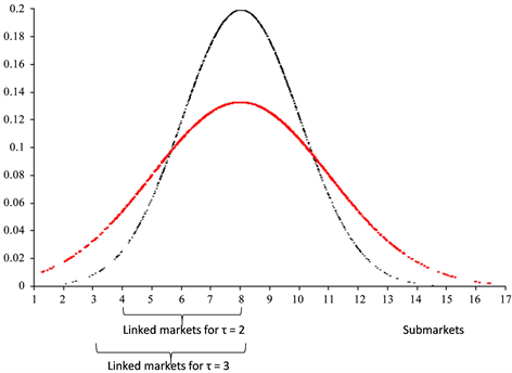
Graph 1. Discovery of submarkets by a lottery process according to a normal function. The vertical axis indicates frequency. Decimal separations with commas.

$V^k={\left[Q_{j{k}^{\prime }}-Q_{jk}\right]}_{j=1,\cdots ,n}$ (3.7)

where $j,k,k^{\prime }$ indicates line j and columns k and $k^{\prime }$ .

Finally, it constructs the matrix $W^k$ with the price differences between two linked submarkets obtained from the matrix $Z^k$ :

$W^k=Z^k{V}^k$ for $k=1,\cdots ,m$ (3.8)

Similarly to Equation (3.2) proposed by Littlechild and Owen, the total variation of supply (of demand, if negative) in each submarket, with agents starting from submarket k, is given by:

$X^k={\left[{\sigma }_j^k\right]}_{j=1,\cdots ,n}{W}^k$ (3.9)

where ${\sigma }_j^k$ is the drafted transfer coefficients.

The total variation of the supply (of the demand, if negative), with agents starting from all the submarkets, is obtained as follows:

$X={\displaystyle {\sum }_{k=1,\cdots ,m}{X}^k}={\displaystyle {\sum }_{k=1,\cdots ,m}{\left[{\sigma }_j^k\right]}_{j=1,\cdots ,n}{W}^k}$ (3.10)

Now it begins of the price formation equation. In the new version of Equation (3.1), the parameter $b_k$ would depend on a deterministic factor and another random factor. The program user informs the deterministic factor d. The random factor is given by the expression: $r^k~unif\left(0,1\right)$ for each $k=1,\cdots ,m$ . Therefore:

$b_k=d\cdot r^k$ (3.11)

The prices practiced in the different submarkets evolve according to the various iterations. The final price in the submarkets, after the first iteration in the loop, is given by:

$p_f^k=p^k-b_k\cdot X\left(:,j\right)$ (3.12)

where $X\left(:,j\right)$ denotes the k-th column of X. For $k=1,\cdots ,m$ .17

For each new iteration in t, $p_i^k\left(t\right)=p_f^k\left(t-1\right)$ , new transfers are generated and the system compares the price distance in t, among the different submarkets, with the minimum allowable M margin (margin of convergence reported by the user):

$\left|p_f^{k^{\prime }}\left(t\right)-p_f^k\left(t\right)\right|<M$ (3.13)

to each $k^{\prime }=1,\cdots ,k-1,k+1,\cdots ,m$

4. Results of the Numerical Simulation

Each simulation involves running the program only once for a set of parameters entered by the user. The program performs several iterations until the reported convergence condition is reached. The first simulation was done for 10 submarkets in which initial prices were drawn by the computer based on Equation (3.3). Prices are placed in increasing order and are associated with sub-markets from 1 to m. The user informs the number n of agents that will act in each submarket (total number of agents $n\times m$ ), the number N of iterations in the program loop (the number of times the arbitrage occurs), the convergence margin M of the prices of different submarkets (maximum permissible final discrepancy), the deterministic factor τ of the alertness coefficient, the deterministic factor d of Equation (11) used as a parameter of the price equation. The values initially reported are m = 10, n = 20, N = 100, M = 1, τ = 5, d = 0.1. Flexibility coefficients ${\sigma }_j^k$ are generated by programs based on a uniform distribution function of 0 to 1 and used in estimating the total supply variation (demand, if negative) in each submarket. Therefore, initially in the face of Equation (3.11), the parameter $b_k$ is drawn for each k. Table 1 shows, for a simulation, the output on the Matlab screen with these coefficients for $n\times m$ agents, as well as the parameters $b_k$ for the price equation determined by the deterministic value d informed and by the draw in the uniform distribution. These values will remain the same throughout any simulation for a given d.

Then, it estimates the Equation (3.4) of the research effort of each agent translated by a normal distribution function around the initial price of the submarket in question. The program through two loops going through all the submarkets and all the agents makes such an estimate. In each case, the draw of a specific point is made throughout the distribution function that governs the price search effort. Table 2 shows the exit of the prices drawn, in the hundredth iteration, around each of the initial prices of the different submarkets. The system reveals, as a result of the draws in question, the submarkets discovered by each of the agents operating in the m submarkets. Such an estimate is made based on Equation (3.5) which translates into a specific programming sequence.

The system generates the $Z^k$ matrix of zeros and 1, which translates linked or discovered markets by agents from all other submarkets. Next, the matrix with the price differences between the submarkets now connected and the submarkets of origin is produced. The next step in the simulation is to estimate the supply variation (demand) in each submarket. This is done with agents starting at the same time from all the submarkets in question. Equation (3.12) is used to estimate the final price in the submarkets after each iteration. From one iteration to another, the system automatically proceeds in the simulation exercise up to the number of them informed. At the end of the hundredth iteration, Table 3 shows the Matlab output with the variation of the supply (demand) in each submarket, for this iteration, by line and by agents starting from different submarkets, and the total variation of the supply in each submarket.18

Table 1. Determining factor of the price function (d), flexibility coefficients drawn ( ${\sigma }_j^k$ ), and parameters drawn for the price equation ( $b_k$ ).

Source: Result of the simulation in Matlab, given the program and parameters provided by the user.

Table 2. Prices drawn around respective initial prices. 100th iteration.

Source: Result of the simulation in Matlab. Prices generated in the hundredth iteration.

Table 3. Results at the end of the 100th iteration. Total net supply in linked markets for each agent in different submarkets. Total net supply for all agents in each submarket. Vectors of initial prices and at the end of the hundredth iteration.

Source: Result of the simulation in Matlab.

It also shows, at the end of it, the final prices, which are compared to the prices initially drawn. In this case, it is the hundredth iteration, because the loop of the program that commands the process of iterative approximation to the margin of convergence reported by the user was executed a hundred times, the N number informed. For different N informed, the number of iterations would have been naturally different.

At the end, a final price vector $p_f$ is given in the table above. It should be noted that, in this case, there was no convergence between prices. However, instead of stating that the convergence process is not possible, the model for different calibration parameters is tested. If it keeps the same parameters of the previous simulation, it now evaluates the simulation model for different alertness coefficients τ, in the values of 10, 15, 20 and 25. In each case, the same coefficients of flexibility ${\sigma }_j^k$ and the same parameters of the price equation is maintained, both in Table 1. The initial price vector is also the same for each simulation involving a specific τ. In all these simulations, it is first necessary to examine the degree of linkage that is obtained between the 10 submarkets in question. To do so, a procedure is developed that generates Table 4 where the number indicates quantities of agents arbitrating the respective submarkets for agents located in the same line (of the 20 lines generated in each submarket), including the agent of origin, which was already in the submarket. Any number greater than 1 indicates, therefore, connection between submarkets.

Table 4. Results of linking submarkets to the end of the 100th iteration. Linked markets and “degree of connection”.

Source: Result of the simulation in Matlab. Hundredth iteration.

These markets are not always directly linked. Market with such link can be seen in the right part of the table for agents departing from submarket 8, which discriminates the markets that he can exploit from that point (which receive the number 1). For agents starting from the submarket in question, there are at most 4 markets directly linked. Other results for linking are found for agents starting from other submarkets. For the given simulation, in the hundredth iteration, the maximum connection that was obtained was 4 markets directly linked to agents starting from the 1 to 8 markets. The program also accuses when no market is linked to another (in the case of agents that depart from markets 9 and 10).

The table to the left of Table 4 is obtained by summing the unit inputs of agents, in the same lines in the table, starting from a certain submarket. The aggregate number should be interpreted as the degree of connection of the submarkets, it indicates the number of agents located in the line of the table, which acts in the linking of a market with some of the others. The last line of the table on the left should be interpreted as the overall degree of linking of the submarket in question to some of the others, considering all the agents that have in the submarket their base.

Note that these tables only relate to the connections obtained in the last iteration, which starts from the price vector established in the penultimate round, since prices are possibly other for each iteration and, therefore, the submarket links. Markets are linked in the round in question, then switched off, and potentially tied again in the next iteration. The connection is not definitive, since the prices practiced in the submarkets change with each iteration and the agents depart again to the process of search of advantageous prices and discovery of opportunities of arbitration every round.

Keeping the same basic parameters, then new simulations were done for different coefficients of alertness τ. We work with the values of 10, 15, 20 and 25. Table 5 shows the degree of linkage of the submarkets to the end of the hundredth iteration for the first and last value. Simulations were also generated for intermediate values.

Table 5. Degree of connection of the submarkets to the end of the 100th iteration. Two coefficients of alertness τ. (d = 0.1).

Source: Result of the simulation in Matlab. Hundredth iteration.

Graph 2 shows the trajectory of prices between submarkets, with the successive discovery of new markets and the arbitrage process, for the different coefficients of alertness applied to the problem under analysis, given the values adopted in the other parameters. In all simulations, the initial prices are the same, by construction, and the final submarket price vector is shown, in the different contexts, in 10 steps equally spaced up to the hundredth iteration.

It should be noted that, even increasing the deterministic coefficient of alertness, homogeneous prices were not obtained in all submarkets considered.

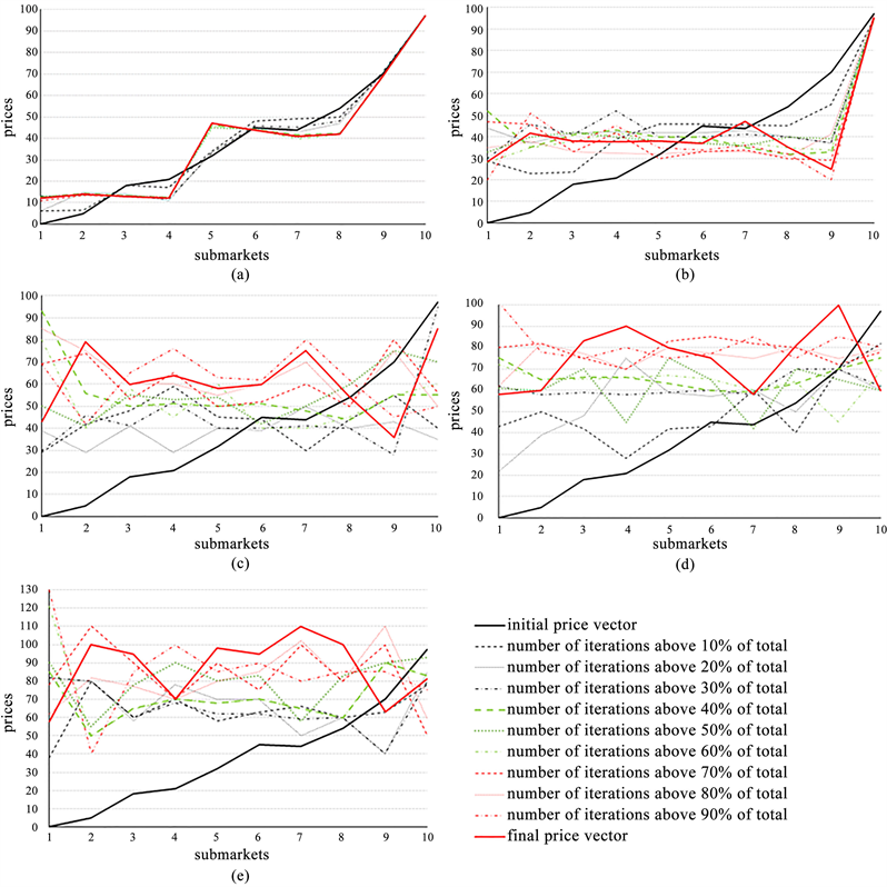
Graph 2. Evolution of submarket prices in 10 steps. Final prices in the 100th iteration. Same initial prices in different simulations. Different coefficients of alertness τ (d = 0.1). (a) τ = 5; (b) τ = 10; (c) τ = 15; (d) τ = 20; (d) 25. Source: Result of the simulation in Matlab, given the program and parameters provided by the user. Output in EXCEL. Hundredth iteration.

Differently from the theoretical statements of Littlechild and Owen [1] , in the simulation exercise there was no price convergence, only that the prices of the different submarkets tend to oscillate in an intermediate price range between the extreme values. Even increasing the value of the alertness, the system does not converge. However, the results of the numerical simulation may be other, and the system behaves dynamically in another way, when the values assigned to the basic parameters change in the exercise. Indeed, by making the deterministic product d of Equation (3.11), which regulates the price formation in Equation (3.12), assume a value less than 0.1, it is observed that the system has a more stable behavior, with the dynamic convergence of submarket prices to the same uniform value. In fact, a new set of graphs with the evolution of submarket prices can be obtained by making, for example, the coefficient d assuming, by calibration, the value of 0.01.

Graph 3 remakes price trajectories in the simulations and presents its evolution in a similar way to that of the previous figure, considering now the new value assigned to the parameter of the price equation. The new figure shows the evolution of the system to the alertness τ assuming values of 5, 10, 15 and 20.

Thus, in this case, uniform prices in the different submarkets are already formed with an alertness coefficient equal to 20. So the convergence process depends on the level of alertness of the entrepreneurs, but also on the parameters of the price equation, of how the new prices respond to the excesses of net supply that are being formed in the submarkets per action of the arbitration process. Table 6 shows the degree of binding of the submarkets to $\tau =10$ and 25 for the purpose of comparing the behavior of the system with the new deterministic factor d of the price equation in 0.01, in relation to the linking results for d = 0.1 of the previous exercise.

It should be noted that with the price equation parameter only 10% of the previous level, not only the convergence of submarket prices in the simulations is guaranteed, but also a considerably greater degree of linkage between the markets. By comparing Table 5 and Table 6, the highest values of connections cues in the case with a lower d and $\tau =25$ are apparent. More precisely, in this case the mean degree of link increases from 123.1 to 194.5. Interestingly, the same does not occur for τ = 10.

Similar simulations were done for even lower values of d. Note that with the deterministic parameter of the price equation very low, say d = 0.001, there is no price convergence for an alertness of 20. In order to evaluate the effect of the factor d on convergence, an exercise is done with a big number of iterations (up to one thousand), and it evaluates the number of iterations that are necessary to allow the convergence of submarket prices to occur in terms of the values assumed by the parameter in question. It assumes in all the exercises that the alertness is 20. Graph 4 shows the relationship between the parameter d of the price equation and the number of iterations for the convergence of submarket prices to occur. The economic interpretation of this graph is that when the coefficient d falls in a range between 0.008 and 0.018, specific to the parameters informed and the simulation exercise in question, convergence occurs in a smaller number of iterations, that is, it is performed more efficiently.

Note that, for $\tau =20$ , there is no price convergence between submarkets, for up to 1.000 iterations, for d = 0.001, and that the convergence occurs rapidly for d = 0.01, according to previous simulations (Graph 4). The range of d between 0.0075 and 0.02 is quite favorable for convergence at homogeneous prices in the simulations, however, such convergence does not occur easily (and may never occur) when d assumes values outside this range. Then the dynamic behavior of the prices in the simulations depends on the calibration of the model. It depends fundamentally on the parameter of the price equation and depends naturally on the alertness τ. Regarding the alertness, it sees in Table 6 how crucial to convergence it is. In fact, a greater degree of alertness facilitates the process of convergence. Next, it is investigated by means of new simulations, to what extent a greater degree of entrepreneurial alertness facilitates the convergence of prices.

Table 6. Degree of connection of the submarkets to the end of the 100th iteration. Two coefficients of alertness τ (d = 0.01).

Source: Result of the simulation in Matlab. Hundredth iteration.

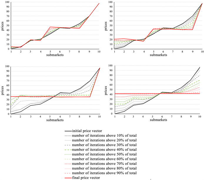
Graph 3. Evolution of submarket prices in 10 stages. Final prices in the 100th iteration. Same initial prices in different simulations. Different coefficients of alertness degree τ (d = 0.01). (a) τ = 5; (b) τ = 10; (c) τ = 15; (d) τ = 20. Source: Result of the simulation in Matlab, given the program and parameters provided by the user. Output in EXCEL. Hundredth iteration.

Graph 4. Relationship between the parameter d of the submarkets price equation and the number of iterations of the program so that price convergence occurs in the stipulated margin of 1. τ = 20. Decimal separations with commas. Source: Result of the simulation in Matlab, given the program and parameters provided by the user. Output in EXCEL.

Graph 5 shows the relationship between τ and the number of iterations required for the convergence of submarket prices. In all simulations d = 0.01 was used. As seen previously, in the simulations, for the alertness below 20, there is no price convergence in the submarkets. The convergence velocity seems increasing for τ increasing up to 50, with some oscillation. However, it is noted that a higher value of the alertness, above this level, does not have a well-defined relation with the speed of price convergence. In fact, by examining the behavior of the curve in Graph 5, it is clear that, from a certain level, a greater degree of entrepreneurial alertness has no systematic effect on convergence. For $50\le \tau \le 200$ , an oscillatory pattern is observed in the relation between τ and convergence velocity. In the next step of the paper, it is analyzed the relationship between the alertness coefficient and processing time until the convergence of prices in the submarkets is reached.

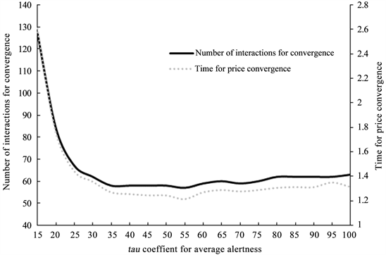
Therefore, it is still worth to examine the dynamic behavior of the numerical simulation model taking into account the processing time of the computer.19 For this exercise, all “pause” commands of the program in Matlab have been deleted. Simulations are performed for up to a thousand iterations, at the end of which the number of iterations for price convergence and the associated time in seconds are computed. For the exercise in question, a new vector of initial prices in the submarkets is drawn. Table 7 shows the output screen of the first simulation again indicating the case of 10 submarkets, 20 agents in each. The new drawn transfer coefficients are shown. The simulation is done initially for deterministic coefficient of alertness of 15. New simulations, with the same basic parameters of this, will be made for different values of τ, from 20 to 100, varying 5.

Graph 5. Relation between the alert level (τ) and the number of iterations of the program in order for price convergence to occur at the stipulated margin of 1 (d = 0.01). Source: Result of the simulation in Matlab, given the program and parameters provided by the user. Output in EXCEL.

Table 7. Number of submarkets (m), number of agents in each (n), deterministic factor of the price function (d), drawn flexibility coefficients ( ${\sigma }_j^k$ ) and drawn parameters for the price equation ( $b_k$ ).

Source: Result of the simulation in Matlab, given the program and parameters provided by the user.

This new vector of initial prices in the submarkets is p_i = (10.9755; 18.7461; 26.6179; 43.2485; 43.2642; 65.5498; 69.4752; 75.8099; 79.7830; 93.3760) and the price vector at the end of the 127th interaction is p_f = (47.9075; 48.0096; 47.3818; 48.0051; 48.1018; 48.8615; 48.0196; 47.9994; 48.0165; 48.0226) for the initial case with $\tau =15$ . The processing time was, in this case, 2.6051 seconds until the convergence of the submarkets prices.

Graph 6 shows the relationship between the alertness (τ) and the convergence process measured by both the number of iterations and the processing time. It should be noted, therefore, that the two indicatives are approximate. For τ between 15 and 35, there is an increase in the convergence velocity at uniform prices, along a convex curve, as measured by the two criteria of number of iterations and time. In the different simulations, starting from $\tau =35$ , the process of dynamic price convergence between submarkets stabilizes, without increasing speed even with increasing values for the degree of alertness.

5. Analysis of the Process of Convergence with Heterogeneous Agents Regarding the Alertness, and Market Barriers

In the simulations made in the previous section, a specific coefficient of flexibility ( ${\sigma }_j^k$ ) is assigned to each agent in accordance with Equation (3.2). However, the agents are homogeneous in relation to the alertness (although the link between markets, for each one, depends on a specific lottery). Thus, it would be natural to examine the behavior of the simulations for heterogeneous agents. Taking into account Kirzner’s theory, expectations are raised that heterogeneous agents with regard to alertness would facilitate the process of convergence. The reason for this will not be explored here, only it does to run the simulation model, with the hypothesis of very different agents regarding the reaction to the markets and alertness. Such changes are incorporated into the Matlab program. Now, instead of a single alertness for all agents, the user reports only the deterministic component of that variable, or the average alertness ( ${\tau }_m$ ). Based on this, the effective level of alertness specific to each agent ( ${\tau }_j$ ), based on Equation (3.14), is calculated:

${\tau }_j={\tau }_m\left(1+0.25{\xi }_j\right)$ . (5.1)

where ${\xi }_j~N\left(0,1\right)$ for each j.

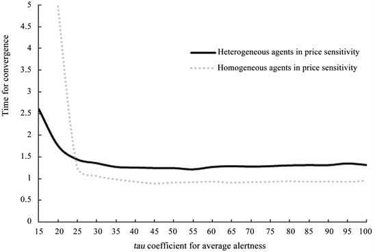
Before the simulation for heterogeneous agents, we observe the behavior for the previous case assuming now homogeneous agents also regarding the coefficient of flexibility in the arbitration Equation (3.2). Therefore, a single value for σ is assumed to be the mean of the coefficients obtained in the previous simulation which is 0.5 (since ${\sigma }_i^j~unif\left(0,1\right)$ ). For this new context, Graph 7 shows the relationship between the alertness and the time for price convergence in the submarkets in cases of homogeneous or heterogeneous agents regarding the transfer rate, the sensitivity to the prices practiced (maintaining homogeneity regarding the alertness.). The simulation is done for d = 0.01.

Note that, unlike Kirzner’s theory of the role of agent heterogeneity, convergence is more rapid for homogeneous agents in the arbitration process. Although it is observed that, for the value of alertness below 25, the convergence is more effective in the case of heterogeneous agents of the previous simulation. Anyway, it is more important to analyze the agents’ heterogeneity regarding the alertness. Based on Equation (5.1), the Matlab program is changed and the simulations are running again.

Graph 6. Relation between the alertness (τ), number of iterations of the program for convergence of prices and convergence time (in seconds). Stipulated margin of one. Source: Result of the simulation in Matlab, given the program and parameters provided by the user. Output in EXCEL.

Graph 7. Relationship between the alertness (τ), and time for price convergence. Stipulated margin of one. Source: Result of the simulation in Matlab, given the program and parameters provided by the user. Output in EXCEL.

Table 8 shows the alertness drawn when the user reports with 15 the average alertness ${\tau }_m$ . In the case, the values drawn were from 5.19 to 24.87. Drawings of this type were made for different values of ${\tau }_m$ from 15 to 100, with variations of 5. In the simulation, the initial price vector is fixed and, according to the single draw made for it, it was established in p_i = (13.8777; 19.6625; 37.5274; 41.9346; 61.0507; 64.0454; 77.2848; 90.9310; 91.5204; 95.3267).

Table 8. Specific values of alertness assigned to each of the 200 agents considered, according to the draw specified in equation (5.1).

Source: Result of the simulation in Matlab. given the program and parameters provided by the user.

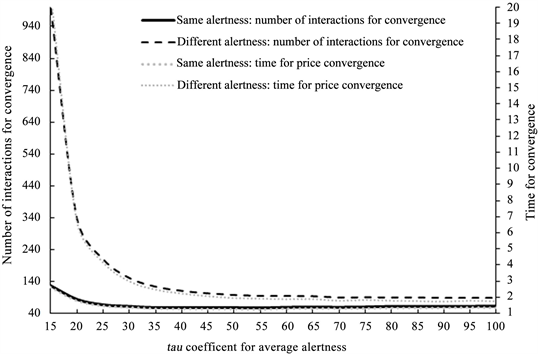
Graph 8 shows the time of convergence to equilibrium, with the arbitration process, comparing the cases with agents of the same alertness with the other of heterogeneous agents in this respect (in both cases, the agents differ as regarding the transfer coefficient). Again, it obtains a result in which the convergence velocity is higher for homogeneous agents, measured in terms of the number of iterations and time. Note, however, that the differences are larger for small values of ${\tau }_m$ , from 15 to 30.

Finally, this paper examines the effect of entry barriers in the process of price convergence of submarkets by arbitrage. Economic market barriers, as it knows, are a cost that agents are required to incur to operate in a given market, a cost that would not exist without the barrier. They can be thought of as artificial obstacles that hamper the arbitrage of markets and make them less efficient, with implications for loss of welfare. There are many ways to model entry barriers and various exercises have been done in that direction. It shows here the results of simulations with a particular strategy of artificially imposing such barriers by slight modifications in the program. Differences in prices between submarkets of origin and those in submarkets discovered by the alertness are result in complete transfer rates, and the respective excess of net supply formed, only when the price differences module between them are less than 10% of the price at the base submarket. For differences above this, it is imposed that only 10% of the transfers are made.

This hypothesis has greater effect in the first iterations, in which the price differences between the submarkets are larger. Then, as prices come closer, the barriers are no longer significant. However, due to the initial difficulty with the transfers, such barriers modify the result of the simulations. In the new exercise, a new set of values drawn for the flexibility coefficients is set. For d = 0.01, and the same basic parameters, simulations are generated for the case with barrier compared to the case without barrier. Differences in the degree of linkage of submarkets in the barrier and non-barrier cases are sensitive. In the first case, prices converge in a much smaller number of iterations and the final degree of market linkage, in the last iteration before convergence, is significantly higher.

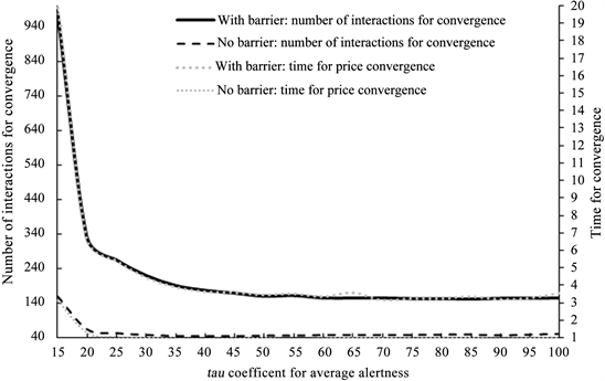
Finally, Graph 9 shows the relationship between the average alertness ( ${\tau }_m$ ) and time for price convergence in the two cases analyzed with and without barriers. Note the intuitive and expected result that the barriers impede the process of price convergence in the submarkets by arbitrage. The number of iterations and the time required for convergence in the case with barriers, as modeled, is much greater. However, we note the interesting result that the differences are greater for smaller coefficients of alertness, which involve a larger number of iterations and a longer processing time.

Graph 8. Relationship between the average alertness ( ${\tau }_m$ ), and time for price convergence. Stipulated margin of one. Source: Result of the simulation in Matlab, given the program and parameters provided by the user. Output in EXCEL.

Graph 9. Relationship between the average alertness ( ${\tau }_m$ ) and time for price convergence. Stipulated margin of one. Source: Result of the simulation in Matlab, given the program and parameters provided by the user. Output in EXCEL.

6. Conclusions

The simulation exercises of this essay solve some shortcomings of the purely mathematical model of reference. Nevertheless, not all the criticisms pointed out in the section (2) in modeling the market process were met, concentrating more on offering new formalization of the discovery mechanism. The biggest advantage is to analyze the market process in an iterative model. It models the discovery process as attempts of uncertain outcome governed by a known probability distribution whose variance is determined by the entrepreneurial alertness. It would not be difficult to extend the simulation model to the general equilibrium treatment. The equilibrium stability can be monitored by observing the numerical results of the simulations in successive attempts. A production model could also be incorporated without much difficulty. In the simulations, non-negativity constraints need not be explicit because the calibration method selects the most appropriate parameters for economically meaningful solutions. One can easily do the alertness coefficient could vary with time. More sophisticated models when the probability of market discovery, using game theory, could be incorporated, and remain as the theme for further studies.

The way the arbitration process was represented in the simulations is more Austrian than the mathematical model of reference in the literature. The discovery process is now explained as governed by a probability regulated by distribution function. Price differences no longer occur only by an unexplained chance. The process of how agent action affects prices is accompanied step by step by an iterative mechanism. Simulations consider agents that act independently, but strategic actions could be incorporated. The greater absence of the proposed simulation model, also present in algebraic treatment, remains a way of treating expectations, always difficult to incorporate into numerical simulation.

In the model presented, it is possible to follow step by step the market process and the conditions under which a uniform price is established. It can be monitored as exogenous changes in the data affect the equilibrium point. Unlike the purely algebraic treatment, in the simulations, explicit calibration techniques of the coefficients of the model are present. A deeper analysis of welfare losses with the absence of entrepreneurial discovery behavior would be lacking, but the entry barrier model allows us to observe the difficulties of price convergence in this context.

The main conclusions reached with numerical simulations are that the model converges well, within an adequate specification of parameters, and that, in this sense, the most important parameters are the alertness (τ) and the coefficient d of the prices function. For $0.005\le d\le 0.02$ and $\tau \ge 20$ , the submarket prices converge well to a uniform value after a number of iterations and processing time. The heterogeneity of the agents did not show much impact for the convergence. Input barriers naturally make convergence less effective. Moreover, such inefficiency can be quantified here.

The idea of using a draw ruled by a normal distribution adequately represents the probabilities of discoveries, the fact that nearby markets are more likely to be discovered. The problem lies in the assumption that, once a submarket has been discovered at a certain distance, given by the computer draw, all the submarkets closest to the initial base of the agent in question would also be revealed. Simulation models do not replace the algebraic treatment, because in them the results are highly dependent on the specification of parameters. The economic sense of these parameters is not always easy to interpret. The convergence efficiency indicators are specified in terms of number of iterations and time of processing. It would be interesting to imagine more concrete situations and think this time in terms of time involved in real processes such as hours and days.

NOTES

¹Lundholm [2] believes that the theoretical model in question uses only the initial ideas of Kirzner, an Austrian school economist, as Kirzner [3] does, and it does not quite describe the author’s insights after 1982 when he incorporates more fundamentally the role of uncertainty. According to the critic, the model, in fact, is not tied to the more recent Austrian description of the market process in which agents discover individual buyers and sellers, not markets. See Kirzner [4] .

²According to the Google Scholar indicator, the paper was cited 41 times since, scientific performance short of a successful study. Moreover, it is noted that it was published in a highly regarded journal (Journal of Economic Theory). Although there is much more mathematics today in Austrian models than in the past, the paper in question did not have the repercussion that was imagined.

³It was present in the classical economists, and Alfred Marshall reiterated it.

⁴In general, these studies are based on a modeling structure with game theory. Keyhani [5] offers an interesting survey of numerical simulation procedures investigating price convergence.

⁵Computer simulations allow us to go beyond analytical treatment and to study systems that cannot be easily modeled with equations.

⁶The term refers to the concept widely used by Kirzner ( [3] , [6] ), which in this author is much richer and full of implications. It concerns the entrepreneur’s role in discovering opportunities and how this leads to market equilibrium. In this explanation, entrepreneurial activity is crucial for the market process to equilibrium. The concept of alertness in Kirzner also incorporates speculative and innovative activities.

⁷There is nothing particularly special about normal function other than the fact that it is a symmetric distribution function and concentrated at the central points. Any other distribution function with this characteristic would also serve our purposes.

⁸The alertness basically affects the discovery of new submarkets. The transfer rates could also be affected by it, however, for simplicity, alertness is considered to affect only the probability of finding out. That is, in the simulations one can change the alertness and the transfer rate independently of each other in order to monitor the effects of each one on the numerical results.

⁹The proof of the theorem depended on the hypothesis that the submarkets in question were linked. In one of the four lemmas related to the demonstration, it is also shown that the difference between the lowest and the highest price tends to zero. In addition, all the prices in the different submarkets approximate an average value (the weighted average price commented above). Cf. Littlechild and Owen [1] .

¹⁰Desktop with processor Intel i7-3770, 3.4 GHz CPU, 8 GB RAM, 64 bit operating system. Matlab version: R2013a.

¹¹The interested reader may have access to the Matlab program used in the simulation on a special webpage.

¹²A numerical simulation study is better suited than purely algebraic to follow the process in which the variables feedback, because the simulations are done in a programming environment that does it step by step, as the values are generated and recalculated.

¹³In this regard, Littlechild and Owen [1] propose that the discovery process be modeled as a Markov chain: “It seems natural to model this discovery process as a markov process, in which the transition probabilities for each trades depend upon (1) the “attractiveness” for him of the markets which remains to be discovered, and (2) his own entrepreneurial ability.” (p. 366) However, the authors do not explain this model.

¹⁴The hypothesis that agent $\left(j,k\right)$ always departs from market k, where he is, implies that he does not memorize the markets that were linked in the previous round. Unlike the reference model, in the simulations there is a forgetting of submarkets with each round. Such a hypothesis is necessary because prices in each one change constantly with the arbitration process itself.

¹⁵The precise identification of the agent depends on j and k. There are n agents operating in each submarket ( $j=1,\cdots ,n$ ) and k submarkets ( $k=1,\cdots ,m$ ), so there would be $n\times m$ agents in total.

¹⁶Of course, the two distances associated with the two distribution tails must be considered.

¹⁷From Equation (3.1), it follows that, at each iteration, $p_f^k-p_i^k=b_k\left(x_i^k-x_f^k\right)$ and therefore $p_f^k=p_i^k-b_k\left(x_f^k-x_i^k\right)$ .

¹⁸By rows, we interpret only movements of the nth agents of each column. Where n represents the location of the line counting vertically from top to bottom. The hundredth iteration corresponds to the maximum number of turns reported in the programming loop.

¹⁹Processing time should be seen as a measure of the efficiency of the price convergence process.

Conflicts of Interest

The authors declare no conflicts of interest.

References

[1]	Littlechild, S.C. and Owen, G. (1980) An Austrian Model of Entrepreneurial Market Process. Journal of Economic Theory, 23, 361-379. https://doi.org/10.1016/0022-0531(80)90018-6
[2]	Lundholm, M. (1987) Information in Economic Theory: An Austrian Approach. Working Paper, n. 188 (Dec.), Uppsala University, Uppsala.
[3]	Kirzner, I.M. (1973) Competition and Entrepreneurship. University of Chicago Press, Chicago.
[4]	Kirzner, I.M. (2011) Market Theory and the Price System. In: Boettke, P.J. and Sautet, F.E., Eds., The Collected Works of Israel M. Kirzner, Liberty Fund, [1963].
[5]	Keyhani, M. (2016) Computer Simulation Studies of the Entrepreneurial Market Process. In: Berger, E.S.C. and Kuckertz, A., Eds., Complexity in Entrepreneurship. Innovation and Technology Research: Applications of Emergent and Neglected Methods, Springer International Publishing, Cham. Switzerland. https://doi.org/10.1007/978-3-319-27108-8
[6]	Kirzner, I.M. (1997) Entrepreneurial Discovery and the Competitive Market Process: An Austrian Approach. Journal of Economic Literature, 35, 60-85.