Mixed Fractional Merton Model to Evaluate European Options with Transaction Costs

Foad Shokrollahi

Department of Mathematics and Statistics, University of Vaasa, Vaasa, Finland.

DOI: 10.4236/jmf.2018.84040                

Abstract

This paper deals with the problem of discrete-time option pricing by the mixed fractional version of Merton model with transaction costs. By a mean-self-financing delta hedging argument in a discrete-time setting, a European call option pricing formula is obtained. We also investigate the effect of the time-step δt and the Hurst parameter H on our pricing option model, which reveals that these parameters have high impact on option pricing. The properties of this model are also explained.

Keywords

Transaction Costs, Mixed Fractional Brownian Motion, European Option, Merton Model

1. Introduction

Over the last few years, the financial markets have been regarded as complex and nonlinear dynamic systems. A series of studies has found that many financial market time series display scaling laws and long-range dependence. Therefore, it has been proposed that the Brownian motion in the classical Black-Scholes (BS) model [1] should be replaced by a process with long-range dependence.

Nowadays, the BS model is the one most commonly used for analyzing financial data, and some scholars have presented modified forms of the BS model which have influential and significant outcomes on option pricing. However, they are still theoretical adaptations and not necessarily consistent with the empirical features of financial return series, such as nonnormality, long-range dependence, etc. For example, some scholars [2] [3] [4] [5] [6] have showed that returns are of long-range (or short-range) dependence, which suggests strong time-correlations between different events at different time scales [7] [8] [9] . In the search for better models for describing long-range dependence in financial return series, a mixed fractional Brownian (MFBM) model has been proposed as an improvement of the classical BS model [10] - [18] . The advantage of using the MFBM is that the markets are free of arbitrage.

Moreover, Cheridito [10] has proved that, for $H\in \left(\frac{3}{4}\mathrm{,1}\right)$ , the MFBM is

equivalent to one with Brownian motion, and hence time-step and long-range dependence in return series have no impact on option pricing in a complete financial market without transaction costs. In addition, a number of empirical studies show that the paths of asset prices are discontinuous and that there are jumps in asset prices, both in the stock market and foreign exchange [9] [19] [20] [21] [22] .

The above researches have an important implication for option pricing. Merton [23] created a revolution in option pricing when the underlying asset was governed by a diffusion process. Based on this theory, Kou [24] , Cont and Tankov [25] also considered the problems of pricing options under a jump diffusion environment in a larger setting. In this paper, to capture jumps or discontinuities, fluctuations and to take into account the long memory property of financial markets, a mixed fractional version of the Merton model is introduced, which is based on a combination of Poisson jumps and MFBM. The mixed fractional Merton (MFM) model is based on the assumption that the underlying asset price is generated by a two-part stochastic process: 1) small, continuous price movements are generated by an MFBM, and 2) large, infrequent price jumps are generated by a Poisson process. This two-part process is intuitively appealing, as it is consistent with an impressive market in which major information arrives infrequently and randomly. This process may provide a description for empirically observed distributions of exchange rate changes that are skewed, leptokurtic, have long memory and fatter tails than comparable normal distributions and apparent nonstationary variance. Further, we will show the impact of the time-step and long-range dependence in return series exactly on option pricing, regardless of whether proportional transaction costs are considered or not in a discrete time setting.

Leland [26] is a pioneer scholar, who investigated option replication where transaction costs exist in a discrete time setting. In this view, the arbitrage-free arguments presented by Black and Scholes [1] are not applicable in a model where transaction costs occur at all moments of trading of the stock or bond. The problem is that perfect replication incurs an infinite number of transaction costs because of the infinite variation which exists in the geometric Brownian motion. In this regard, a delta hedge strategy is constructed in accordance with revision conducted a discrete number of times. Transaction costs lead to the failure of the no arbitrage principle and the continuous time trade in general: instead of no arbitrage, the principle of hedge pricing, according to which the price of an option is defined as the minimum level of initial wealth needed to hedge the option, comes into force.

According to the empirical findings obtained before and the views of behavioral finance and econophysics, we are motivated to examine the problem that exists in option pricing, while the dynamics of price $S_t$ follows a mixed fractional jump-diffusion process under the transaction costs. We assume that $S_t$ satisfies

$S_t=S_0{\text{e}}^{\mu t+\sigma B\left(t\right)+{\sigma }_H{B}_H\left(t\right)+N_t\ln J}.$ (1.1)

where $S_0\mathrm{,}\mu \mathrm{,}\sigma$ and ${\sigma }_H$ are fixed; $B\left(t\right)$ is a Brownian motion; $B_H\left(t\right)$ is a

fractional Brownian motion with Hurst parameter $H\in \left(\frac{3}{4}\mathrm{,1}\right)$ ; $N_t$ is a Poisson

process with intensity $\lambda >0$ ; and J is a positive random variable. We assume that $B\left(t\right)\mathrm{,}{B}_H\left(t\right)\mathrm{,}{N}_t$ and J are independent.

This paper is organized into several sections. In Section 2, we will study the problem of option pricing with transaction costs by applying delta hedging strategy. In addition, a new framework for pricing European option is obtained when the stock price $S_t$ is satisfied in Equation (1.1). Section 3 is devoted to empirical studies and simulations to show the performance of the MFM model. A conclusion is presented in Section 4.

2. Pricing Option by Mixed Fractional Version of Merton Model with Transaction Costs

Suppose ${\left\{B\left(t\right)\right\}}_{t\ge 0}$ be a standard Brownian motion and ${\left\{B_H\left(t\right)\right\}}_{t\ge 0}$ be a fractional Brownian motion with the Hurst parameter $H\in \left(\frac{3}{4}\mathrm{,1}\right)$ , both defined

on complete probability space $\left(\Omega \mathrm{,}F\mathrm{,}{F}_t\mathrm{,}P\right)$ , the absolute price jump size J is a nonnegative random variable drawn from lognormal distribution, i.e. $\ln \left(J\right)=N\left({\mu }_J,{\sigma }_J\right)$ , which implies

$J~Lognormal\left({\text{e}}^{{\mu }_J+\frac{{\sigma }_J^2}{2}}\mathrm{,}{\text{e}}^{2{\mu }_J+{\sigma }_J^2}\left({\text{e}}^{{\sigma }_J^2}-1\right)\right)$

and a Poisson process $N={\left(N_t\right)}_{t\ge 0}$ with rate $\lambda$ . Additionally, the processes $B\mathrm{,}{B}_H\mathrm{,}N$ and J are independent, P is the real world probability measure and ${\left(F_t\right)}_{t\in \left[\mathrm{0,}T\right]}$ denotes the P-augmentation of filtration generated by $\left(B\left(\tau \right)\mathrm{,}{B}_H\left(\tau \right)\right)\mathrm{,}\tau \le t$ .

The objective of this section is to derive a stock pricing formula under transaction costs in a discrete time setting. Consider $\left(D\mathrm{,}S\right)$ -market with a bond $D_t$ and a stock $S_t$ , where

$D_t=D_0{\text{e}}^{rt}\mathrm{.}$ (2.1)

and

$S_t=S_0{\text{e}}^{\mu t+\sigma B\left(t\right)+{\sigma }_H{B}_H\left(t\right)+N_t\ln J},\mu ,\sigma ,{\sigma }_H\in R,D_0,S_0,t\in R^{+}.$ (2.2)

The groundwork of modeling the effects of transaction costs was done by Leland [26] . He adopted the hedging strategy of rehedging at every time-step $\delta t$ . That is, with every $\delta t$ the portfolio is rebalanced, whether or not this is optimal in any sense. In the following proportional transaction cost option pricing model, we follow the other usual assumptions in the Black-Scholes model, but with the following exceptions:

1) The price $S_t$ of the underlying stock at time t satisfies Equation (2.2).

2) The portfolio is revised every $\delta t$ where $\delta t$ is a finite and fixed, small time-step.

3) Transaction costs are proportional to the value of the transaction in the underlying. Let k denote the round trip transaction cost per unit dollar of transaction. Suppose $U>0$ shares are bought $\left(U>0\right)$ or sold $\left(U<0\right)$ at the price $S_t$ , then the transaction cost is given by $\frac{k}{2}\left|U\right|S_t$ in either buying or selling, where k is a constant. The value of k will depend on the individual investor. In the MFM model, where transaction costs are incurred at every time the stock or the bond is traded, the no arbitrage argument used by Black and Scholes no longer applies. The problem is that due to the infinite variation of the MFBM, perfect replication incurs an infinite amount of transaction costs.

4) The hedge portfolio has an expected return equal to that from an option. This is exactly the same valuation policy as earlier on discrete hedging with no transaction costs.

5) Traditional economics assumes that traders are rational and maximize their utility. However, if their behaviour is assumed to be boundedly rational, the traders' decisions can be explained both by their reaction to the past stock price, according to a standard speculative behaviour, and by imitation of other traders’ past decisions, according to common evidence in social psychology. It is well known that the delta-hedging strategy plays a central role in the theory of option pricing and that it is popularly used on the trading floor. Therefore, based on the availability heuristic, suggested by Tversky and Kahneman [27] , traders are assumed to follow, anchor, and imitate the Black-Scholes delta-hedging strategy to price an option. In this case, delta-hedging argument is a partial and imperfect hedging strategy, which does not eliminate all of the risk. However, as mentioned in the paper [28] , in most models of stock fluctuations, except for very special cases, risk in option trading cannot be eliminated and strict arbitrage opportunities do not exist, whatever be the price of the option. The risk cannot be eliminated is furthermore the fundamental reason for the very existence of option markets.

Delta hedging is an options strategy that aims to reduce, or hedge, the risk associated with price movements in the underlying asset, by offsetting long and short positions. For example, a long call position may be delta hedged by shorting the underlying stock. This strategy is based on the change in premium, or price of option, caused by a change in the price of the underlying security. In this section we use the delta hedging strategy to obtain a pricing formula for European call option.

Let the price of European call option be denoted with expiration T and strike price K by $C\left(t\mathrm{,}{S}_t\right)$ with boundary conditions:

$C\left(T,S_T\right)={\left(S_T-K\right)}^{+},C\left(t,0\right)=0,C\left(t,S_t\right)\to S_t\text{as}{S}_t\to \infty .$ (2.3)

Then, $C\left(t\mathrm{,}{S}_t\right)$ is derived by the following theorem.

Theorem 2.1. The price at every $t\in \left[\mathrm{0,}T\right]$ of a European call option with strike price K that matures at time T is given by

$C\left(t,S_t\right)={\displaystyle \underset{n=0}{\overset{\infty }{\sum }}}\frac{{\text{e}}^{-{\lambda }^{\prime }\left(T-t\right)}{\left({\lambda }^{\prime }\left(T-t\right)\right)}^n}{n!}\left[S_t\varphi \left(d_1\right)-K{\text{e}}^{-r\left(T-t\right)}\varphi \left(d_2\right)\right].$ (2.4)

Moreover, $C\left(t,S_t\right)$ satisfies the following equation

$\begin{array}{l}\frac{\partial C}{\partial t}+r{S}_t\frac{\partial C}{\partial S_t}+\frac{S_t^2{\hat{\sigma }}^2}{2}\frac{{\partial }^{2}C}{\partial S_t^2}-rC+\lambda E\left[C\left(t\mathrm{,}J{S}_t\right)-C\left(t\mathrm{,}{S}_t\right)\right]\\ -\lambda E\left[J-1\right]S_t\frac{\partial C}{\partial S_t}=\mathrm{0,}\end{array}$ (2.5)

where

$d_1=\frac{\ln \left(\frac{S_t}{K}\right)+r_n\left(T-t\right)+\frac{{\sigma }_n^2}{2}\left(T-t\right)}{{\sigma }_n\sqrt{T-t}},d_2=d_1-{\sigma }_n\sqrt{T-t},$ (2.6)

${\lambda }^{\prime }=\lambda E\left(J\right)=\lambda {\text{e}}^{{\mu }_J+\frac{{\sigma }_J^2}{2}},{\sigma }_n^2={\hat{\sigma }}^2+\frac{n{\sigma }_J^2}{T-t},$ (2.7)

$r_n=r-\lambda E\left(J-1\right)+\frac{n\ln E\left(J\right)}{T-t}=r-\lambda \left({\text{e}}^{{\mu }_J+\frac{{\sigma }_J^2}{2}}-1\right)+\frac{n\left({\mu }_J+\frac{{\sigma }_J^2}{2}\right)}{T-t},$ (2.8)

${\hat{\sigma }}^2={\sigma }^2+{\sigma }_H^2{\left(\delta t\right)}^{2H-1}+k\sqrt{\frac{2}{\text{π}}\left(\frac{{\sigma }^2}{\delta t}+{\sigma }_H^2{\left(\delta t\right)}^{2H-2}\right)}sign\left(\Gamma \right),$ (2.9)

$sign\left(\Gamma \right)$ is the signum function of $\frac{{\partial }^{2}C}{\partial S_t^2}$ ; n is the number of prices jumps;

$\delta t$ is a small and fixed time-step; k is the transaction costs and $\varphi \left(\mathrm{.}\right)$ is the cumulative normal distribution.

Moreover, using the put call parity, we can easily obtain the valuation model for a put currency option, which is provided by the following corollary.

Corollary 2.1. The value of European put option with transaction costs is given by

$P\left(t,S_t\right)={\displaystyle \underset{n=0}{\overset{\infty }{\sum }}}\frac{{\text{e}}^{-{\lambda }^{\prime }\left(T-t\right)}{\left({\lambda }^{\prime }\left(T-t\right)\right)}^n}{n!}\left[K{\text{e}}^{-r\left(T-t\right)}\varphi \left(-d_2\right)-S_t\varphi \left(-d_1\right)\right].$

3. Properties of Pricing Formula

In this section, we present the properties of MFM’s log-return density. The effects of Hurst parameter and time-step on our modified volatility $\left({\sigma }_n^2\right)$ are also discussed in the discrete time and continuous time cases. Then we show that these parameters play a significant role in a discrete time setting, both with and without transaction costs.

3.1. Log-Return Density

In the case of MFM the log return jump size is assumed to be $\left(Y_i\right)=\left(\ln J_i\right)~N\left({\mu }_J,{\sigma }_J^2\right)$ and the probability density of log return $x_t=\ln \left(S_t/S\right)$ is achieved as a quickly converging series of the following form:

$P\left(x_t\in A\right)={\displaystyle \underset{n=0}{\overset{\infty }{\sum }}}P\left(N_t=n\right)P\left(x_n\in A|N_t=n\right)$

$P\left(x_t\right)={\displaystyle \underset{n=0}{\overset{\infty }{\sum }}}\frac{{\text{e}}^{-\lambda t}{\left(\lambda t\right)}^n}{n!}N\left(x_t;\mu t+n{\mu }_J,{\sigma }^{2}t+{\sigma }_H^2{t}^{2H}+n{\sigma }_J^2\right),$ (3.1)

where

$\begin{array}{l}N\left(x_t\mathrm{<mo>\; ;\; </mo>}\mu t+n{\mu }_J\mathrm{,}{\sigma }^{2}t+{\sigma }_H^2{t}^{2H}+n{\sigma }_J^2\right)\\ =\frac{1}{\sqrt{2\text{π}\left({\sigma }^{2}t+{\sigma }_H^2{t}^{2H}+n{\sigma }_J^2\right)}}exp\left[-\frac{{\left(x_t-\left(\mu t+n{\mu }_J\right)\right)}^2}{2\left({\sigma }^{2}t+{\sigma }_H^2{t}^{2H}+n{\sigma }_J^2\right)}\right]\end{array}$ (3.2)

The term $P\left(N_t=n\right)=\frac{{\text{e}}^{-\lambda t}{\left(\lambda t\right)}^n}{n!}$ is the probability that the asset price jumps

n times during the time interval of length t. And $P\left(x_n\in A|N_t=n\right)=N\left(x_t;\mu t+n{\mu }_J,{\sigma }^{2}t+{\sigma }_H^2{t}^{2H}+n{\sigma }_J^2\right)$ is the mixed fractional normal density of log-return. It supposes that the asset price jumps i times in the time interval of t. As a result, in the MFM model, the log-return density can be described as the weighted average of the mixed fractional normal density by the probability that the asset price jumps n times.

The outstanding properties of log-return density $P\left(x_t\right)$ are observed in the MFM. Firstly, the ${\mu }_J$ sign refers to the expected log-return jump size, $E\left(Y\right)=E\left(\ln J\right)={\mu }_J$ , which indicates the skewness sign. If ${\mu }_J<0$ , the log-return density $P\left(x_t\right)$ shows negatively skewed, and if ${\mu }_J=0$ , it is symmetric as displayed in Figure 1 (Table 1).

Secondly, larger value of intensity $\lambda$ (which means that jumps are expected to occur more frequently) makes the density fatter-tailed as illustrated in Figure 2. Note that the excess kurtosis in the case $\lambda =20$ is much smaller than in the case $\lambda =1$ or $\lambda =10$ . This is because excess kurtosis is a standardized measure (by standard deviation) (Table 2).

3.2. The Impact of Parameters

Mantegna and Stanley [29] as pioneer scholars proposed the scaling invariance method from the complex science of economic systems which led to numerous investigations into scaling laws in finance. The major question in economics is whether the price impact of scaling law and long-range dependence is significant in option pricing. The answer to this question is assured. For instance, one of the significant issues in finance concerning the modeling of high-frequency data is related to analyzing the volatility in different time scales.

Figure 1. MFM’s log-return density. Fixed parameters are $\sigma =0.25$ , ${\sigma }_H=0.25$ , $H=0.76$ , ${\sigma }_J=0.1$ , ${\mu }_J=0$ , $\mu =0.009$ , and $t=0.5$ .

Figure 2. MFM’s log-return density. Fixed parameters are $\sigma =0.25$ , ${\sigma }_H=0.25$ , $H=0.76$ , ${\sigma }_J=0.1$ , $\lambda =3$ , $\mu =0.009$ , and $t=0.5$ .

Table 1. Annualized moments of Merton’s log-return density in Figure 1.

Table 2. Annualized moments of Merton’s log-return density in Figure 2.

Remark 3.1. In a continuous time setting $\left(\delta t=0,\lambda \ne 0\right)$ without transaction costs the implied volatility is ${\hat{\sigma }}_n^2={\sigma }^2+\frac{n{\sigma }_J^2}{T-t}$ , thus the option value is similar to

the Merton jump diffusion model [19] . Moreover, if $\delta t=0$ in the absence of transaction costs and jump case, the MFM model reduces to the BS model

$\frac{\partial C}{\partial t}+r{S}_t\frac{\partial C}{\partial S_t}+\frac{S_t^2{\sigma }^2}{2}\frac{{\partial }^{2}C}{\partial S_t^2}-rC=0,$ (3.3)

which shows that the Hurst parameter H and time-step $\delta t$ have no effect on option pricing model in a continuous time setting $\left(\delta t=0\right)$ .

Remark 3.2. In a discrete time setting without transaction costs $\left(k=0,\delta t\ne 0\right)$ , if jump occurs, the modified volatility is

${\hat{\sigma }}_n^2={\sigma }^2+{\sigma }_H^2{\left(\delta t\right)}^{2H-1}+\frac{n{\sigma }_J^2}{T-t}$ and when jump does not occur $\left(\lambda =0\right)$ , from Equation (2.5), we have

$\frac{\partial C}{\partial t}+r{S}_t\frac{\partial C}{\partial S_t}+\left({\sigma }^2+{\sigma }_H^2{\left(\delta t\right)}^{2H-1}\right)\frac{S_t^2}{2}\frac{{\partial }^{2}C}{\partial S_t^2}-rC=0,$ (3.4)

which demonstrates that the delta hedging strategy in a discrete time case is fundamentally different in comparison with a continuous time case. It also indicates that the scaling exponent $2H-1$ and time-step $\delta t$ play a significant role in option pricing theory. Figure 3 illustrates the impacts of the time-step, Hurst parameter, mean jump, and jump intensity on our option pricing model.

Remark 3.3. From [30] we infer there exists $\delta t\in \left(\mathrm{0,}\frac{1}{M}\right)$ such that

$\underset{\delta t\in \left(\mathrm{0,}\frac{1}{M}\right)}{min}{\hat{\sigma }}^2\mathrm{,}$ (3.5)

Holds,

where $M>1$ , k is small enough

${\hat{\sigma }}^2={\sigma }^2+{\sigma }_H^2{\left(\delta t\right)}^{2H-1}+k\sqrt{\frac{2}{\text{π}}\left(\frac{{\sigma }^2}{2\delta t}+{\sigma }_H^2{\left(\delta t\right)}^{2H-2}\right)}.$ (3.6)

Indeed,

$\begin{array}{l}{\sigma }_H^2{\left(\delta t\right)}^{2H-1}+k\sqrt{\frac{2}{\text{π}}\left(\frac{{\sigma }^2}{\delta t}+{\sigma }_H^2{\left(\delta t\right)}^{2H-2}\right)}\\ \ge 2{\sigma }_H{\left(\delta t\right)}^{H-\frac{1}{2}}{k}^{\frac{1}{2}}{\left(\frac{2}{\text{π}}\left(\frac{{\sigma }^2}{\delta t}+{\sigma }_H^2{\left(\delta t\right)}^{2H-2}\right)\right)}^{\frac{1}{4}}\mathrm{.}\end{array}$ (3.7)

Figure 3. Modified volatility. Fixed parameters are $\sigma =0.1$ , ${\sigma }_H=0.1$ , $H=0.76$ , ${\sigma }_J=0.03$ , $T=0.2$ , $T=0.2$ , and $t=0.1$ .

Set

${\sigma }_H^2{\left(\delta t\right)}^{2H-1}=\sqrt{\frac{2k^2}{\text{π}}\left(\frac{{\sigma }^2}{\delta t}+\frac{{\sigma }_H^2}{{\left(\delta t\right)}^{2-2H}}\right)}\mathrm{.}$ (3.8)

Thus

${\sigma }_H^2{\left(\delta t\right)}^{2H}=\frac{\frac{2k^2}{\text{π}}+\sqrt{{\left(\frac{2k^2}{\text{π}}\right)}^2+\frac{8k^2}{\text{π}}{\sigma }^2\delta t}}{2}\mathrm{.}$ (3.9)

Suppose

$f\left(x\right)={\sigma }_H^2{x}^{2H}-\frac{\frac{2k^2}{\text{π}}+\sqrt{{\left(\frac{2k^2}{\text{π}}\right)}^2+\frac{8k^2}{\text{π}}{\sigma }^{2}x}}{2}\mathrm{.}$ (3.10)

Since $f\left(0\right)<0$ and

$f\left(\frac{1}{M}\right)={\sigma }_H^2{\left(\frac{1}{M}\right)}^{2H}-\frac{\frac{2k^2}{\text{π}}+\sqrt{{\left(\frac{2k^2}{\text{π}}\right)}^2+\frac{8k^2}{\text{π}}{\sigma }^2\frac{1}{M}}}{2}>0,$ (3.11)

as k is small enough.

Hence, there exists a $\delta t\in \left(\mathrm{0,}\frac{1}{M}\right)$ such that $mi{n}_{\delta t\in \left(\mathrm{0,}\frac{1}{M}\right)}{\hat{\sigma }}^2$ holds.

Suppose

${\hat{\sigma }}^2\left(min\right)=\underset{\delta t\in \left(\mathrm{0,}\frac{1}{M}\right)}{min}{\hat{\sigma }}^2\mathrm{,}$ (3.12)

so

${\sigma }_n^2\left(\min \right)=\underset{\delta t\in \left(0,\frac{1}{M}\right)}{\min }{\sigma }_n^2=\underset{\delta t\in \left(0,\frac{1}{M}\right)}{\min }{\hat{\sigma }}^2+\frac{n{\delta }^2}{T-t}.$ (3.13)

Then the minimal price of an option with respect to transaction costs is displayed as $C_{min}\left(t\mathrm{,}{S}_t\right)$ with ${\sigma }_n^2\left(min\right)$ in Equation (2.4). $C_{min}\left(t\mathrm{,}{S}_t\right)$ can be applied to the real price of an option.

4. Conclusion

To capture the long memory and discontinuous property, this article focuses on the problem of pricing European option in a mixed fractional Merton environment without using the arbitrage argument. We obtain a mixed fractional version of Merton model for pricing European option with transaction costs. Some properties of mixed fractional Merton’s log-return density are discussed. Moreover, we derive that the Hurst parameter H and time-step $\delta t$ play a significant role in pricing option in a discrete time setting for cases both with and without transaction costs. But these parameters have no impact on option pricing in a continuous time setting.

Appendix

Proof of Theorem 2.1. We consider a replicating portfolio with $\psi \left(t\right)$ units of financial underlying asset and one unit of the option. Then, the value of the portfolio at time t is

$P_t=\psi \left(t\right)S_t-C\left(t,S_t\right).$ (4.1)

Now, the movement in $S_t$ and $P_t$ is considered under discrete time interval $\delta t$ . In view of this, we suppose that trading takes place at the specific time points of t and $t+\delta t$ . It can be said that the number of shares through the use of delta-hedging strategy and the present stock price $S_t$ are constantly held during the rebalancing interval $\left[t\mathrm{,}t+\delta t\right)$ . Then, the movement in the value of the portfolio after time interval $\delta t$ is defined as follows:

$\delta P_t=\psi \left(t\right)\delta S_t-\delta C\left(t,S_t\right)-\frac{k}{2}\left|\delta \psi \left(t\right)\right|S_t.$ (4.2)

where $\delta S_t$ is the movement of the underlying stock price, $\delta \psi \left(t\right)$ is the movement of the number of units of stock held in the portfolio, and $\delta P_t$ is the change in the value of the portfolio.

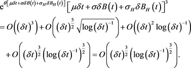
Since the time-step $\delta t$ and the asset change are both small, according to Taylor’s formulae we have if $\delta N_t=0$ with probability $1-\lambda \delta t$ , so

$\begin{array}{c}\delta S_t=S_t\mu \delta t+S_t\delta \sigma B\left(t\right)+S_t\delta {\sigma }_H{B}_H\left(t\right)+\frac{S_t}{2}{\left(\mu \delta t+\sigma \delta B\left(t\right)+{\sigma }_H\delta B_H\left(t\right)\right)}^2\\ +\frac{S_t}{6}{\text{e}}^{\theta \left[\mu \delta t+\sigma \delta B\left(t\right)+{\sigma }_H\delta B_H\left(t\right)\right]}{\left(\mu \delta t+\sigma \delta B\left(t\right)+{\sigma }_H\delta B_H\left(t\right)\right)}^3,\end{array}$ (4.3)

where, and.

Since and are continuous, then from [28] we have

(4.4)

(4.5)

(4.6)

and

Thus, we can get

(4.7)

(4.8)

(4.9)

and

(4.10)

If with probability and the jump of in is assumed to occur at current time t, then

(4.11)

(4.12)

(4.13)

(4.14)

(4.15)

(4.16)

where.

Based on the above assumptions iv and v, we have, i.e.. Then

i.e.

where the current stock price is given. Since

(4.17)

and, from Equations (4.1) - (4.17), we can get

(4.18)

Hence, we assume that

(4.19)

Note that the term is nonlinear, except when does not change sign for all. Since it represents the degree of

mishedging of the portfolio, it is not surprising to observe that is involved in the transaction cost term. We may rewrite Equation (4.19) in the form which resembles the Merton equation:

(4.20)

where and the implied volatility is given by

(4.21)

If, Equation (4.20) becomes mathematically ill-posed. This occurs when and. However, it is known that is always positive for the simple European call and put options in the absence of transaction costs. If we postulate the same sign behaviour for in the presence of transaction costs, Equation (4.20) becomes linear under such an assumption so that the Merton formula becomes applicable except that the modified volatility should be used as the volatility parameter. Moreover, if from Equation (4.20) we obtain

where

is the signum function of, is a small and fixed time-step, k is the transaction costs and is the cumulative normal distribution.

Conflicts of Interest

The authors declare no conflicts of interest.

References

[1]	Black, F. and Scholes, M. (1973) The Pricing of Options and Corporate Liabilities. The Journal of Political Economy, 81, 637-654. https://doi.org/10.1086/260062
[2]	Willinger, W., Taqqu, M.S. and Teverovsky, V. (1999) Stock Market Prices and Long-Range Dependence. Finance and Stochastics, 3, 1-13. https://doi.org/10.1007/s007800050049
[3]	Ozdemir, Z.A. (2009) Linkages between International Stock Markets: A Multivariate Long-Memory Approach. Physica A: Statistical Mechanics and Its Applications, 388, 2461-2468. https://doi.org/10.1016/j.physa.2009.02.023
[4]	Mariani, M., Florescu, I., Varela, M.B. and Ncheuguim, E. (2009) Long Correlations and Levy Models Applied to the Study of Memory Effects in High Frequency (Tick) Data. Physica A: Statistical Mechanics and Its Applications, 388, 1659-1664. https://doi.org/10.1016/j.physa.2008.12.038
[5]	Sottinen, T. and Valkeila, E. (2003) On Arbitrage and Replication in the Fractional Black-Scholes Pricing Model. Statistics & Decisions/International Mathematical Journal for Stochastic Methods and Models, 21, 93-108.
[6]	Sottinen, T. and Viitasaari, L. (2016) Pathwise Integrals and Itô-Tanaka Formula for Gaussian Processes. Journal of Theoretical Probability, 29, 590-616. https://doi.org/10.1007/s10959-014-0588-2
[7]	Cajueiro, D.O. and Tabak, B.M. (2007) Long-Range Dependence and Multifractality in the Term Structure of Libor Interest Rates. Physica A: Statistical Mechanics and Its Applications, 373, 603-614. https://doi.org/10.1016/j.physa.2006.04.110
[8]	Cajueiro, D.O. and Tabak, B.M. (2007) Long-Range Dependence and Market Structure. Chaos, Solitons & Fractals, 31, 995-1000. https://doi.org/10.1016/j.chaos.2005.10.077
[9]	Mandelbrot, B.B. and Stewart, I. (1998) Fractals and Scaling in Finance. Nature, 391, 758-758.
[10]	Cheridito, P. (2001) Mixed Fractional Brownian Motion. Bernoulli, 7, 913-934. https://doi.org/10.2307/3318626
[11]	Mishura, Y.S. and Valkeila, E. (2002) The Absence of Arbitrage in a Mixed Brownian-Fractional Brownian Model. Trudy Matematicheskogo Instituta imeni VA Steklova, 237, 224-233.
[12]	Mishura, I.S. and Mishura, Y. (2008) Stochastic Calculus for Fractional Brownian Motion and Related Processes. Vol. 1929, Springer Science & Business Media, Kyiv. https://doi.org/10.1007/978-3-540-75873-0
[13]	Shokrollahi, F. and Kılıçman, A. (2014) Pricing Currency Option in a Mixed Fractional Brownian Motion with Jumps Environment. Mathematical Problems in Engineering, 2014, 13.
[14]	Shokrollahi, F. and Kılıçman, A. (2015) Actuarial Approach in a Mixed Fractional Brownian Motion with Jumps Environment for Pricing Currency Option. Advances in Difference Equations, 2015, 1-8. https://doi.org/10.1186/s13662-015-0590-8
[15]	Shokrollahi, F. and Kılıçman, A. (2014) Delta-Hedging Strategy and Mixed Fractional Brownian Motion for Pricing Currency Option. Mathematical Problems in Engineering, 501, Article ID: 718768.
[16]	Shokrollahi, F., Kılıçman, A. and Magdziarz, M. (2016) Pricing European Options and Currency Options by Time Changed Mixed Fractional Brownian Motion with Transaction Costs. International Journal of Financial Engineering, 3, 1650003.
[17]	Xiao, W.-L., Zhang, W.-G., Zhang, X. and Zhang, X. (2012) Pricing Model for Equity Warrants in a Mixed Fractional Brownian Environment and Its Algorithm. Physica A: Statistical Mechanics and Its Applications, 391, 6418-6431. https://doi.org/10.1016/j.physa.2012.07.041
[18]	Cont, R. (2005) Long Range Dependence in Financial Markets. In: Fractals in Engineering, Springer, Berlin, 159-179.
[19]	Merton, R.C. (1976) Option Pricing When Underlying Stock Returns Are Discontinuous. Journal of Financial Economics, 3, 125-144. https://doi.org/10.1016/0304-405X(76)90022-2
[20]	Jarrow, R. and Rosenfeld, E. (1988) Jump Risks and Intemporal Capital Asset Pricing Model. The Journal of Business, 57, 337-351. https://doi.org/10.1086/296267
[21]	Ball, C.A. and Torous, W.N. (1985) On Jumps in Common Stock Prices and Their Impact on Call Option Pricing. The Journal of Finance, 40, 155-173. https://doi.org/10.1111/j.1540-6261.1985.tb04942.x
[22]	Shokrollahi, F. and Kılıçman, A. (2016) The Valuation of Currency Options by Fractional Brownian Motion. Springer Plus, 5, 1145. https://doi.org/10.1186/s40064-016-2784-2
[23]	Merton, R.C. (1973) Theory of Rational Option Pricing. The Bell Journal of Economics and Management Science, 4, 141-183.
[24]	Kou, S.G. (2002) A Jump-Diffusion Model for Option Pricing. Management Science, 48, 1086-1101. https://doi.org/10.1287/mnsc.48.8.1086.166
[25]	Cont, R. and Tankov, P. (2003) Calibration of Jump-Diffusion Option-Pricing Models: A Robust Nonparametric Approach. Journal of Computational Finance, 7, 1-49. https://doi.org/10.21314/JCF.2004.123
[26]	Leland, H.E. (1985) Option Pricing and Replication with Transactions Costs. The Journal of Finance, 40, 1283-1301. https://doi.org/10.1111/j.1540-6261.1985.tb02383.x
[27]	Tversky, A. and Kahneman, D. (1973) Availability: A Heuristic for Judging Frequency and Probability. Cognitive Psychology, 5, 207-232.
[28]	Wang, X.-T., Yan, H.-G., Tang, M.-M. and Zhu, E.-H. (2010) Scaling and Long-Range Dependence in Option Pricing III: A Fractional Version of the Merton Model with Transaction Costs. Physica A: Statistical Mechanics and Its Applications, 389, 452-458. https://doi.org/10.1016/j.physa.2009.09.044
[29]	Mantegna, R.N. and Stanley, H.E. (1995) Scaling Behaviour in the Dynamics of an Economic Index. Nature, 376, 46-49. https://doi.org/10.1038/376046a0
[30]	Wang, X.-T., Zhu, E.-H., Tang, M.-M. and Yan, H.-G. (2010) Scaling and Long-Range Dependence in Option Pricing II: Pricing European Option with Transaction Costs under the Mixed Browni-an-Fractional Brownian Model. Physica A: Statistical Mechanics and Its Applications, 389, 445-451. https://doi.org/10.1016/j.physa.2009.09.043