Dependence of the Yield of Alfalfa on Plant Density and Diet

Alizade Alibala, Zamanov Pasha, Zamanova Azada, Iskenderov Subaxat

Institute of Soil Science and Agrochemistry of ANAS, Baku, Azerbaijan.

DOI: 10.4236/ajps.2017.811183                

Abstract

In this study, under conditions of enclosed soil, experiments were conducted on the dependence of the yield (weight of green mass) of alfalfa (Medicago) on plant density and diet. The experiments were carried out in five variants, in different values of the integrated density of plants and lasted 89 days. As a feed, specially prepared bio fertilizer was used and added with the calculation of 1 kg per 1 m² of area. In the corresponding control variants, bio fertilizer was not used. Analysis of the experimental results showed that the feeding regime made it possible to obtain a maximum yield at higher integral density. At the same time, the increase in the weight of green mass when using bio fertilizers was about 36%.

Keywords

Yield, Density of Standing, Integral Density, Competition between Neighbors, Weight of Green Mass, Differential Density, Biofertilizer, Cultivated Plant, Diet, Arable Fields

1. Introduction

Yield dependence (in some cases the weight of green mass) of the plant population has been widely discussed in the classical papers [1] - [6] . However, there is a view that the yield on the equivalent of one plant tends to a constant value.

$W=\frac{Y}{\rho }=\frac{a}{\rho +b}$ (1)

where W―the yield on the equivalent of one plant; a and b―predetermined constant; ρ―density of scalar plants. The desire for a constant value of the parameter W is connected that, when a relatively small plant density is no competition between plants. It is necessary to think, however that the resulted statement if А-M²―the area of the food for one plant that

$A=\frac{1}{\rho }$ (2)

and replacement of ρ in the equation gives

$W=\frac{aA}{1+BA}$ (3)

This equation allows us to make the following conclusions. For large values of A (small competition) coming mass in average per plant it is substantially constant. On the other hand the

$\frac{\text{d}D}{\text{d}T}=k$ (4)

yield depends on the rate of development of plants. Under the development rate is understood the rate at which varies D―quantitative measure development.

At each stage of the parameter D perceives its index eats

$D\to D_G;D_V;D_R;D_S$ (5)

where G―the process of germination; V―vegetative growth; R―reproductive growth; S―aging.

Attempts to establish a direct link between the growth of culture and its yield, on the one hand, and the various aspects of climate, weather and environment, on the other hand made repeatedly. In this case, the following objectives: explain fluctuations in yields, to identify factors that have these fluctuations the most noticeable effect, and finally armed with the said information, choose a form of management that would allow to manage those factors that can be either raised productivity, or to reduce the total cost.

All of these factors (managed and controlled) play an important role in the formation of productivity. One of the most important control parameters directly related to the productivity of the plant is the average density (number of plants per 1 m²).

The yield depends strongly on the competition saying precisely the competitive survival between plants.

The results confirm that, the size of the role of plants in the competition is this relatively large that species suffer from high density mortality. A deeper analysis of intraspecific plant growth depending on the density of standing is linked to the development of the theory of plant competition [7] [8] .

Large species itself sufficient to lower densities than smaller species and smaller species are very capable to invade toward the unused space [9] .

The ability to inhibit the growth of its neighbors, and the ability to resist the inhibition of growth are widely regarded as two forms of competition: competitive effect and competitive response [10] .

Elaborating on the above we can see the dependence of crop yields on certain parameters which are divided into two groups―both managed and unmanaged

$Y=Y\left(P,\rho ,T,\upsilon ,g,h,R\right)$ (6)

where P nutrient regime which is characterized by several interrelated parameters;

ρ―density of standing scalar;

T―temperature averaged over short intervals of time of observation;

v―wind velocity directed perpendicular to the direction of the series;

g―frequency precipitation averaged over short intervals direction;

h―level rainfall averaged over short intervals of observation;

R―soil type which is characterized by several interrelated parameters.

In the simplest case we can consider the function

$Y=Y\left(M_x{P}_{y}K,\rho \right)$

Then the task is reduced such a density of standing that will allow you to get the maximum yield with the possible minimum costs for agro technical activities [11] [12] .

2. Subjects and Methods

2.1. Experimental Procedure

The experiments were conducted in a greenhouse. Closed soil conditions allow you to clearly regulate the impact of external factors such as temperature, solar radiation, wind, etc.

Lucerne (Medicágo) plant was chosen for the experiment―Plants alfalfa genus of annual and perennial grasses and dwarf shrubs of the legume family (Fabaceae). The root system is powerful. The importance of this plant is that it is used in agriculture as a livestock feed. Another important characteristic of this plant is that it is equivalent to the green mass yield.

Experiments were carried out in five embodiments have the following meanings plant density: I variant―S₁ (the average distance between two neighboring plants in one row) 10 cm; S₂ (the average distance between rows) 10 sm; II S₁ = 8.3 sm embodiment; S₂ = 8.3 sm; III variant of S₁ = 6.25 sm; S₂ = 6.25 sm; IV variant S₁ = 5 sm; S₂ = 5 sm; V S₁ = 4 sm embodiment; S₂ = 4 sm.

Simultaneous change of S₁ and S₂ in the direction of the increase is due to the fact that the increase characteristic area A plant belonging to one and showing the limits of its competition with the neighboring four plants. Each option corresponds to a control under the option. Location plant and the characteristic distance between them in the control sub-embodiment was taken as a basically identical to the embodiment. Location experimental sites located in the glass-covered ground are shown in this schematic. It should be noted that each “mini” experimental platform to provide “micro” drainage system. The drainage system of each site was connected to the total drainage of the experimental site.

The total area of all areas amounted to the next value

Width = 2.0 m × 2 + 0.5 m = 4.5 m

Length = 2.0 m × 5 + 0.5 m × 4 = 12.0 m

In order to achieve an identical condition for all the “mini” experimental sites, the soil of the experimental site to a depth of 30 cm was buried and imported outside some distances from the greenhouse construction. For the litter of the general experimental site, special soil was prepared, very similar in its parameters, to soil characteristic of the given terrain. Homogeneously prepared soil for the background had a composition of nutrients; Humus 1.0% - 1.5%; Nitrogen compound―20 mg/kg; Phosphorus―8 mg/kg; Potassium―6 mg/kg. The size of the total experimental area was equal to

$S=\text{4}.\text{5}\text{m}\times \text{12}.0\text{m}=\text{54}{\text{m}}^{\text{2}}$

Adding specially prepared biofertilizer before planting seeds for all five variants were the same and the calculation of 10 tons per 1 hectare (for one embodiment 4 kg per 1 m² - 1 kg)

In this case, the control options are the same. The regime of irrigation and care within the established agro technical measures for all options was identical.

The process of growth of alfalfa plants (Medicágo) in all variants lasted 89 days (March 2―start of the experiment, 29 May―conclusion of the experiment). In the process of growth, the height of the plant was repeatedly measured and this index was averaged. At the end of the experiment in the control variant plant height reached maximum 58 - 60 sm. The maximum height of the plants with the use of bio-fertilizer reaches 65 - 67 cm.

Given that, in this experiment, the “yield” is regarded as the green mass of all the one with each 1 m²―square individually, i.e. for each option for weighing four stacks have been prepared. To collect the green mass produced cut the stem of each plant at a height of 5 - 6 cm from the surface of the soil. Then each pile (total stack 4) are weighed separately and defined “experimental” density of plants according to the following formula.

$\bar{\rho }=\frac{{\displaystyle \underset{i=1}{\overset{4}{\sum }}{\rho }_i}}{4}$ (7)

2.2. Methods of Determining the Density of Plants

Methods of determining the density of the plants was as follows. If the length of the pilot section is equal to L, the width of the land area L₂ would be equal to L₁ × L₂ = sm². If the number of planted trees on a plot of equal N, then

$\frac{N}{S}=\frac{N}{L_1{L}_2}$ (8)

Integral density of plants that is the number of a plant per 1 m² will be equal to

${\rho }_{\mathrm{int}}=\frac{N}{L_1{L}_2}$ (9)

Here ${\rho }_{\mathrm{int}}$ ―the integrated density of the plants. To more accurately determine the density of the plants, between integral and differential averaged densities of plants taken averaged average density.

$\bar{\rho }=\frac{{\rho }_{\mathrm{int}}+{\rho }_{ав}}{2}$ (10)

where ${\rho }_{ав}$ ―averaged differential density; $\bar{\rho }$ ―average mean density.

The average differential density is determined by the following procedure. The participation of various experimental field (different plots is determined by random sampling) is selected small areas with a size of 1 m² and is considered the number of plants in these little squares.

To ensure minimum statistical sample number of small squares should life between 6 and 10 (i = 6 - 10; ρ = ρ_i).

Plant density is determined for each randomly selected section with dimensions of 1 m² ρ_i plants called differential density is determined by the following formula:

${\rho }_{ав}=\frac{{\displaystyle \underset{i=1}{\overset{n}{\sum }}{\rho }_i}}{n}$ (11)

where n―number of selected small areas on the total area. At the same time planting the plants must comply with the following scheme.

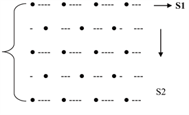
As seen from this scheme L₁ = K₁S₁; L₂ = K₂S₂

Here

S₁―the average distance between two adjacent plants in the same row.

S₂―the average distance between rows.

K₁―the number of plants in the same row.

K₂―the number of rows in the experimental field.

If the total number of plants in the selected field is equal to the N

$N=K_1\times K_2$ (12)

If we write the formula for the ${\rho }_{\mathrm{int}}$

${\rho }_{\mathrm{int}}=\frac{N}{L_1{L}_2}=\frac{K_1\cdot K_2}{K_1{S}_1\cdot K_2{S}_2}$ (13)

Then the density $\bar{\rho }$ is described in this model will take the following form

$\bar{\rho }=\frac{\frac{1}{S_1{S}_2}+{{\displaystyle \sum }}^{\text{}}i{\rho }_i}{2}$ (14)

2.3. Systematization and Processing of Experimental Data

In experimental and control variants (5 variants with application of biofertilizer, 5 variants of control), the density of planting is taken as follows (see Table 1).

For each variant (variant + control) after collection determined weight green mass.

The average weight of the collected green mass in relative units is shown in Table 2. It should be noted that the transition to relative ones to dimensionless units at the first approximation for the ordinate of the OY axis increases the informative and generalization of the results obtained.

Table 1. Density of planting in experimental and control variants.

*) In each embodiment (+control) the distance between the plants in one row and the distance between rows was taken equally, i.e. change in the same way and touched S₁ and S₂; *)) Since the current division in this embodiment is not turned, leaving a very small amount of the free area.

Table 2. Averaged the entire green mass.

The results are presented in graphical form in Figure 1, Figure 2.

As seen from Table 2 and presented drawings maximum by weight green mass when making bio-fertilizer shifted value of about 256 ρ = (S₁ = S₂ = 6.25 sm) k ρ = 400 (S₁ = S₂ = 5 cm).

This situation is related to the fact that, with a relative increase of nutrients reduce competition between nearest neighbors.

Simultaneously, as shown in Table 2 and Figure 1, Figure 2, increase in yield is the weight of the green mass, which is (ratio between the maximum values) (127 − 81): 27% = 36%.

3. Results and Discussion

Ensuring the growth and maintenance of the yield of cultivated plants using environmentally friendly bio-fertilizer is today an important issue solution that will ensure food security. It is necessary to note the fact that, when making mineral fertilizers the soil side mastered Male about 50% nitrogen, 20% - 25% Male phosphorous and 30% potassium Male. Residue remaining in place (nitrogen) remains in the soil, mixed with water or vaporizes as ammonia gas Phosphorus and Kalium remains stable form in the soil. Complex fertilizer contains at only 48% of nutrients. And the remaining 52% is the ballast remains in soluble form in the soil and contaminate it. It should be noted that, the plant takes from one hectare of soil cover each year for 70 - 80 kg of nitrogen; 25 - 30 kg of phosphorus, 60 - 70 kg of potassium and this impoverishes the soil.

Figure 1. Results of the experiment: control option.

Figure 2. Results of the experiment: the use of biofertilizers.

In this paper the example supplied with alfalfa experiment under greenhouse traced two directions: biofertilizer with yield increase (green mass of 1 m² area) and achieve additional gain factor yields via finding optimum plant stand between plants.

It is necessary to consider that finding the optimum plant density for each cultivated plants in large arable fields under external soil climatic conditions and at specified resource capabilities (with the exclusion of parameters S₁ and S₂ which will involve a change in the number of seeds or seedlings) can play an important role in the increase yield and thereby can enhance the economic viability of agricultural production.

The data obtained figures that finding the optimum plant stand of plants cultivated on a large arable field, conducting appropriate agro-technical measures, taking into account this factor may provide a significant economic effect.

4. Conclusions

1) For scalar value, alfalfa plant density was determined in the control variant standing weight maximum which corresponds to the collected green mass. In control embodiment fertilizer was not applied, specially prepared soil nutrients had a composition: 1.0% - 1.5% humus; nitrogen compound―20 mg/kg; phosphorus―8 mg/kg; potassium―6 mg/kg.

2) Leaving standing thickness the same as the respective embodiments, the control application as a result of a specially prepared biofertilizer with calculation of 1 kg per 1 m², and simultaneously increased weight green mass and plant density integrated maximum shifted to right side to increase the integral density ρ. This is due to the fact that the increase in the proportion of nutrients reduced the degree of competition between the neighbors. Yield increase vs eating weight increase of green mass in the application of biofertilizer was approximately 36% (calculation done for maximum points).

Acknowledgements

This work has been executed in Institute of Soil Science and Agrochemistry of the National Academy of Sciences of Azerbaijan and was supported by the Science Development Foundation under the President of the Republic of Azerbaijan―Grant No. EİF-KETPL-2-2015-1(25)-56/38/3-M-38.

Conflicts of Interest

The authors declare no conflicts of interest.

References

[1]	Willey, R.W. and Heath, S.B. (1969) Plant Population and Crop Yield. Advances in Agronomy, 21, 281-321. https://doi.org/10.1016/S0065-2113(08)60100-5
[2]	Thornley, J.H.M. (1983) Crop Yield and Planting Density. Annals of Botany, 52, 257-259. https://doi.org/10.1093/oxfordjournals.aob.a086571
[3]	Berry, G. (1967) A Mathematical Model Relating Plant Yield with Arrangement for Regularly Spaced Crops. Biometrics, 23, 505-515. https://doi.org/10.2307/2528011
[4]	Lib, W.A.R. (2000) Competition along a Nutrient Gradient. Ecological Research, 15, 293-306.
[5]	Shirtliffe, S.J. and Johnston, A.M. (2002) Yield-Density Relationships and Optimum Plant Populations in Two Cultivars of Solid-Seeded Dry Bean (Phaseolus vulgaris L.) Grown in Saskatchewan. Canadian Journal of Plant Science, 82, 521-529. https://doi.org/10.4141/P01-156
[6]	Firbank, L.G. and Watkinson, A.R. (1985) On the Analysis of Competition within Two-Species Mixtures of Plants. Journal of Applied Ecology, 22, 503-517. https://doi.org/10.2307/2403181
[7]	Schamp, B.S. and Aarssen, L.W. (2014) Plant Species Size and Density-Dependent Effects on Growth and Survival. Journal of Vegetation Science, 25, 657-667. https://doi.org/10.1111/jvs.12135
[8]	Aarssen, L.W., Schamp, B.S. and Pither, J. (2006) Why Are There So Many Small Plants? Implications for Species Coexistence. Journal of Ecology, 94, 569-580. https://doi.org/10.1111/j.1365-2745.2006.01128.x
[9]	Schamp, B.S. and Aarssen, L.W. (2010) The Role of Plant Species size Invisibility: A Field Experiment. Oecologia, 162, 995-1004. https://doi.org/10.1007/s00442-009-1499-2
[10]	Wang, P., Stieglitz, T., Zhou, D.W. and Cahill, J.F. (2010) Are Competitive Effect and Response Two Sides of the Same Coin, or Fundamentally Different? Functional Ecology, 24, 196-207. https://doi.org/10.1111/j.1365-2435.2009.01612.x
[11]	Orudzheva, N.I., Babayev, M.P. and Isgandarov, S.M. (2014) Dependence of the Plant Productivity on Optimal Food Regime and Density. American Journal of Plant Sciences, 5, 436-441. https://doi.org/10.4236/ajps.2014.54057
[12]	Orudzheva, M., Babayev, P., Isgandarov, S.M. and Alizade, A. (2013) Influence of the Plant Density on Productivity. Soil-Water Journal, 2, 1021-1028.