1. Introduction
We encounter higher dimensions in String Theory and its derivatives. Let us examine how and under what conditions we encounter these higher dimensions. Our starting point is from the very beginnings of Quantum Theory.
According to Dirac we cross over from Classical Physics to Quantum Physics once we realize that there is no infinite precision in measuring physical quantities [1] . This prescription applies to both non relativistic and relativistic Quantum Mechanics.
Let us now carry over this prescription to a measurement of spacetime coordinates. That is we consider the scenario where we cannot go down to spacetime points. In other words there would be a minimum scale of precision. These ideas were considered some decades ago in attempts to overcome infinities and divergences. In this context it was shown a long time ago by H.S. Snyder [2] that such a prescription would lead to the following noncommutative geometry:
 (1)
(1)
where l is the minimum infinitesimal length. (1) can be further simplified to
 (2)
(2)
(cf. Refs. [2] - [5] ). Now  is the minimum time scale.
In other words, as can be concluded from (1) and (2) the coordinates are no longer scalars rather they would be susceptible to a quarternionic description, with coordinates being represented by matrices. This can be seen directly from (2) (cf. Ref. [3] ).
2. Non Commutativity
There is some physics that is hidden in the above―we have to consider time as being no longer unidirectional but going backward and forward, as can be modelled by a two Wiener process [6] .
We first define the forward and backward velocities corresponding to having time going forward and backward (or positive or negative time increments) in the usual manner,
 (3)
(3)
This leads to the Fokker-Planck equations

 (4)
(4)
defining
 (5)
(5)
We get on addition and subtraction of the equations in (4) the equations
 (6)
(6)
 (7)
(7)
It must be mentioned that V and U are the statistical averages of the respective velocities. We can then introduce the definitions
 (8)
(8)
 (9)
(9)
We next observe the decomposition of the Schrodinger wave function as
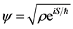
leads to the well known Hamilton-Jacobi type equation
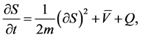 (10)
(10)
where

From (8) and (9) we can finally deduce the usual Schrodinger equation or (10) [6] .
We note that in this formulation three conditions are assumed, conditions whose import has not been clear. These are [7] :
(1) The current velocity is irrotational. Thus, there exists a function  such that

(2) In spite of the fact that the particle is subject to random alterations in its motion there exists a conserved energy, defined in terms of its probability distribution.
(3) The diffusion constant is inversely proportional to the inertialmass of the particle, with the constant of proportionality being a universal constant  (cf. Ref. [7] ):
![]()
We note that the complex feature above disappears if the fractal or non-differential character is not present, (that is, the forward and backward time derivatives (5) are equal): Indeed the fractal dimension 2 also leads to the real coordinate becoming complex. What distinguishes Quantum Mechanics is the adhoc feature, the diffusion constant ![]() in Nelson’s theory and the “Quantum potential” Q of (10) which appears in Bohm’s theory [5] as well, though with a different meaning.
in Nelson’s theory and the “Quantum potential” Q of (10) which appears in Bohm’s theory [5] as well, though with a different meaning.
Interestingly from the Uncertainty Principle,
![]()
we get back the equation of Brownian motion. This shows the close connection on the one hand, and provides, on the other hand, a rationale for the particular, otherwise adhoc identification of ![]() above―its being proportional to
above―its being proportional to![]() .
.
We would like to emphasize that we have arrived at the Quantum Mechanical Schrodinger equation from Classical considerations of diffusion, though with some new assumptions. In the above, effectively we have introduced a complex velocity ![]() which alternatively means that the real coordinate
which alternatively means that the real coordinate ![]() goes into a complex coordinate
goes into a complex coordinate
![]() (11)
(11)
To see this in detail, let us rewrite (5) as
![]() (12)
(12)
where we have introduced a complex coordinate X with real and imaginary parts ![]() and
and ![]() $, while at the same time using derivatives with respect to time as in conventional theory.
$, while at the same time using derivatives with respect to time as in conventional theory.
We can now see from (5) and (12) that
![]() (13)
(13)
That is, in this non relativistic development either we use forward and backward time derivatives and the usual space coordinate as in (5), or we use the derivative with respect to the usual time coordinate but introduce complex space coordinates as in (11).
We know that
![]()
means that the four dimensional rotational group goes over into the Minkowski formulation [8] , as it leads to the invariant Minkowski metric,
![]() (14)
(14)
which is invariant.
There is another way of looking at this. As has been pointed out by Sachs [9] if we generalize (11) to three dimensions we come to not three but four dimensions and a quarternionic description
![]()
Or equivalently
![]() .
.
Remarkably the same Minkowski invariant element is recovered, using the algebra of the Pauli matrices [4] . Not surprisingly there is a lack of spacetime reflection symmetry in this formulation, because the forward backward time of (3) and subsequent equations are not carrying this symmetry.
In summary the above two Wiener process leads to a special relativistic formulation. This description of time is hidden in Special Relativity.
There is another way in which we can come to the same conclusion. We first define a complete set of base states by the subscript ![]() and
and ![]() the time elapse operator that denotes the passage of time between instants
the time elapse operator that denotes the passage of time between instants ![]() and
and![]() ,
, ![]() greater than
greater than![]() . We denote by,
. We denote by, ![]() , the amplitude for the state
, the amplitude for the state ![]() to be in the state
to be in the state ![]() at time t, and [5] [10]
at time t, and [5] [10]
![]()
We can now deduce from the super position of states principle that,
![]() (15)
(15)
and finally, in the limit,
![]() (16)
(16)
where the matrix ![]() is identified with the Hamiltonian operator. We have argued earlier at length that (16) leads to the Schrodinger equation [5] [10] . In the above we have taken the usual unidirectional time to deduce then on relativistic Schrodinger equation. If however we consider a Wiener process in (15) then we will have to consider instead of (16)
is identified with the Hamiltonian operator. We have argued earlier at length that (16) leads to the Schrodinger equation [5] [10] . In the above we have taken the usual unidirectional time to deduce then on relativistic Schrodinger equation. If however we consider a Wiener process in (15) then we will have to consider instead of (16)
![]() (17)
(17)
which then in the limit can be seen to lead to the relativistic Klein-Gordon equation, rather than the Schrodinger type diffusion equation which comes from (15).
It is interesting that this same description of the spacetime coordinates in terms of the Pauli matrices, as in the quarternionic description above can be recovered from the noncommutative relations from (1) and (2).
It may be remembered that this oscillation of time between positive and negative increment values takes place at the micro scale. This leads to an interesting pictorial description in terms of modernfield theory: if “![]() ” would describe anti particles, this would mean that a particle would essentially be accompanied by a swarm of anti particles.
” would describe anti particles, this would mean that a particle would essentially be accompanied by a swarm of anti particles.
3. Discussion
It thus appears that the universe in this formulation is multidimensional as in String and other Quantum Gravity theories as the coordinates now become multi component objects. The question that arises is how or why do we come down to our usual 3 + 1 dimensions? An answer can be found in the noncommutative formulation given in (2) where the coordinates x, y, z, and t turn up in terms of Pauli matrices. This formulation in (2) reduces to the usual Quantum theory―though not the relativistic Quantumtheory―if the order of l2 can be neglected where l is the fundamental length. Retaining order of l2 leads to relativity and the description in terms of the Pauli matrices or the quarternionic description. From a geometrical point of view as has been discussion in detail [3] [4] , order of l2 represents a quantum of area of Quantum Gravity approaches. When this area becomes a line segment we come down to the usual Minkowski universe.
So in summary the higher dimensional quantum of area appears at very high energies. At these ultra high energies the Dirac and Klein-Gordon equations get modified― one way this can be done was worked out by the author (cf. Ref. [4] ). At lower energies we have the Minkowski world and the Dirac equation and the Klein-Gordon equation of Special Relativity and finally at even lower energies we have the usual space and time and the Schrodinger equation.
Finally it may be remarked that at ultra high energies, the Cini-Toushek formulation comes into play rather than the Foldy-Wothuysen (lower energy) one. This has been considered in detail by the author [11] . The interesting consequence is that these particles display neutrino like properties―apparent masslessness and handedness. Perhaps we can consider some neutrinos to be luminal heavier particles.