On the Performances of Classical VAR and Sims-Zha Bayesian VAR Models in the Presence of Collinearity and Autocorrelated Error Terms

M. O. Adenomon, V. A. Michael, O. P. Evans

Department of Mathematics & Statistics, The Federal Polytechnic, Bida, Nigeria.

DOI: 10.4236/ojs.2016.61012                

Abstract

In time series literature, many authors have found out that multicollinearity and autocorrelation usually afflict time series data. In this paper, we compare the performances of classical VAR and Sims-Zha Bayesian VAR models with quadratic decay on bivariate time series data jointly influenced by collinearity and autocorrelation. We simulate bivariate time series data for different collinearity levels (﹣0.99, ﹣0.95, ﹣0.9, ﹣0.85, ﹣0.8, 0.8, 0.85, 0.9, 0.95, 0.99) and autocorrelation levels (﹣0.99, ﹣0.95, ﹣0.9, ﹣0.85, ﹣0.8, 0.8, 0.85, 0.9, 0.95, 0.99) for time series length of 8, 16, 32, 64, 128, 256 respectively. The results from 10,000 simulations reveal that the models performance varies with the collinearity and autocorrelation levels, and with the time series lengths. In addition, the results reveal that the BVAR4 model is a viable model for forecasting. Therefore, we recommend that the levels of collinearity and autocorrelation, and the time series length should be considered in using an appropriate model for forecasting.

Keywords

Vector Autoregression (VAR), Classical VAR, Bayesian VAR (BVAR), Sims-Zha Prior, Collinearity, Autocorrelation

Received 3 September 2015; accepted 22 February 2016; published 25 February 2016

1. Introduction

There are various objectives for studying time series. These include the understanding and description of the generated mechanism, the forecasting of future value and optimum control of a system [1] . In time series literature, many authors have found out that multicollinearity and autocorrelation usually afflict time series data. For instance, Gujarati [2] observed that multicollinearity problem usually afflicted the VAR models. It was reported that correlation coefficients was an appropriate indicator when collinearity began to severely distort model estimation and subsequent prediction [3] . In a recent work of Garba et al. [4] , they observed that the autocorrelation problem usually afflicted time series data. Lastly, Adenomon and Oyejola [5] studied the performances of VAR and BVAR model (assuming harmonic decay) when the bivariate time series were jointly influenced by collinearity and autocorrelation.

The aim of this study is to examine the performances of the classical VAR and Sims-Zha Bayesian VAR model in the presence of collinearity and autocorrelated error terms.

2. Model Description

2.1. Vector Autoregression (VAR) Model

Given a set of k time series variables, , VAR models of the form

(1)

provide a fairly general framework for the Data General Process (DGP) of the series. More precisely this model is called a VAR process of order p or VAR(p) process. Here is a zero mean independent white noise process with non singular time invariant covariance matrix ∑_u and the A_i are (k × k) coefficient matrices. The process is easy to use for forecasting purpose though it is not easy to determine the exact relations between the variables represented by the VAR model in Equation (1) above [6] .

Also, polynomial trends or seasonal dummies can be included in the model.

The process is stable if

(2)

In that case it generates stationary time series with time invariant means and variance covariance structure. The basic assumptions and properties of a VAR processes is the stability condition. A VAR(p) processes is said to be stable or fulfills stability condition, if all its eigenvalues have modulus less than 1 [7] .

Therefore To estimate the VAR model, one can write a VAR(p) with a concise matrix notation as:

(3)

Then the Multivariate Least Squares (MLS) for B yields

(4)

2.2. Bayesian Vector Autoregression with Sims-Zha Prior

In recent times, the BVAR model of Sims and Zha [8] has gained popularity both in economic time series and political analysis. The Sims-Zha BVAR allows for a more general specification and can produce a tractable multivariate normal posterior distribution. Again, the Sims-Zha BVAR estimates the parameters for the full system in a multivariate regression [9] .

Given the reduced form model

The matrix representation of the reduced form is given as:

We can then construct a reduced form Bayesian SUR with the Sims-Zha prior as follows. The prior means for the reduced form coefficients are that B₁ = I and. We assume that the prior has a conditional structure that is multivariate Normal-inverse Wishart distribution for the parameters in the model. To estimate the coefficients for the system of the reduced form model with the following estimators

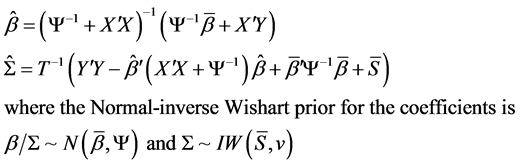
This representation translates the prior proposed by Sims and Zha form from the structural model to the reduced form ([10] [9] ), and ([8] [11] ).

The summary of the Sims-Zha prior is given in Table 1.

3. Simulation Procedure

The simulation procedure is as follows:

Step 1: We generated an artificial two-dimensional (Bivariate data) VAR (2) process that obeys the following form:

such that and where and. Our choice here is similar to the work and illustration of Cowpertwait, [12] . We considered ten autocorrelated levels as . Our choice for this form model is to obtain a stable process and a VAR process with a true lag length [13] .

Step 2: We then use the Cholesky Decomposition to apply to the data generated in Step 1 in order to create a bivariate time series data so that y₁ and y₂ have the desired correlation level [14] . We considered ten multicollinearity levels as.

The combination of Step 1 and 2 therefore produce a bivariate time series such that y₁ and y₂ are jointly influenced by multicollinearity and autocorrelation.

The simulated data assumed time series lengths of 8, 16, 32, 64, 128 and 256. A sample of simulated data is presented in Table 2 below.

3.1. Model Specification

The time series were generated data using a VAR model with lag 2. The choice here is to obtain a bivariate time series with the true lag length. While the VAR and BVAR models of lag length of 2 was used for modeling and forecasting purpose.

Table 1. Hyperparameters of Sims-Zha reference prior.

Source: Brandt and Freeman, [10] .

Table 2. Sample of simulated data for T = 8.

For the BVAR model with Sims-Zha prior, we considered the following range of values for the hyperparameters given below and the Normal-inverse Wishart prior was employed.

We considered two tight priors and two loose priors as follows:

where nµ is prior degrees of freedom given as m + 1 where m is the number of variables in the multiple time series data. In work nµ is 3 (that is two (2) time series variables plus 1 (one)).

Our choice of Normal-inverse Wishart prior for the BVAR models follow the work of Kadiyala & Karlsson, [15] that Normal Wishart prior tends to performed better when compared to other priors. In addition Sims and Zha, [8] proposed Normal-inverse Wishart prior because of its suitability for large systems while Breheny, [16] reported that the most advantage of Wishart distribution is that it guaranteed to produce positive definite draws. Our choice of the overall tightness is in line with work of Brandt, Colaresi and Freeman, [17] . In this work we assumed that the bivariate time series follows a quadratic decay. The Quadratic Decay (QD) model has many attractive theoretical properties that is why it is been applied to many fields of endeavour ([18] [19] ) [20] .

The following are the criteria for Forecast assessments used:

1) Mean Absolute Error (MAE) has a formular. This criterion measures deviation from the

series in absolute terms, and measures how much the forecast is biased. This measure is one of the most common ones used for analyzing the quality of different forecasts.

2) The Root Mean Square Error (RMSE) is given as where y_i is the time series data and y^f is the forecast value of y [13] .

For the two measures above, the smaller the value, the better the fit of the model [21] .

In this simulation study, where N = 10,000. Therefore, the model with the minimum RMSE and MAE result as the preferred model.

3.2. Statistical Packages (R)

In this study three procedures in the R package will be used. They are: Dynamic System Estimation (DSE) [22] ; the vars [23] , and the MSBVAR [24] .

4. Results and Discussion

The Root Mean Square Error (RMSE) and Mean Absolute Error (MAE) were obtained for the various models in the work and are presented in Appendix A, while the ranks are presented in Appendix B. But here the preferred models with respect to their rank are presented. The preferred model for the time series length of 8, 16, 32, 64, 128 and 256 are presented in Tables 3-8 respectively.

In Table 3 below, when T = 8 the BVAR models are preferred in all levels of collinearity and autocorrelation. Also in Table 4 below, when T = 16 the BVAR models are preferred in all levels of collinearity and autocorrelation.

In Table 5 below, when T = 32 the BVAR models are preferred in all levels of collinearity and autocorrelation except in few cases where classical VAR is preferred. In Table 6 below, when T = 64 the BVAR models are preferred in all levels of collinearity and autocorrelation except in some cases where classical VAR is preferred.

In Table 7 below, when T = 128 the BVAR models are preferred in some levels of collinearity and autocorre-

Table 3. Preferred model at different levels of collinearity and autocorrelation when T = 8.

lation and the classical VAR is preferred in some levels of collinearity and autocorrelation. In Table 8 below, when T = 256 the BVAR models are preferred in some levels of collinearity and autocorrelation and the classical VAR is preferred in some levels of collinearity and autocorrelation.

Table 4. Preferred model at different levels of collinearity and autocorrelation when T = 16.

Table 5. Preferred model at different levels of collinearity and autocorrelation when T = 32.

Table 6. Preferred model at different levels of collinearity and autocorrelation when T = 64.

Table 7. Preferred model at different levels of collinearity and autocorrelation when T = 128.

Table 8. Preferred model at different levels of collinearity and autocorrelation when T = 256.

Table 9. Performance ratings of the classical VAR and Sims-Zha Bayesian VAR.

In Table 9 above, the ratings of the model are compared. For short term time series the BVAR4 model dominate except when T = 8 using the MAE criterion, the BVAR1 model dominate. In the medium term and long term, the BVAR4 model dominated using both criteria. This result revealed that the BVAR4 model is a viable model for forecasting.

5. Conclusion and Recommendation

This work examines the performances of classical VAR and Sims-Zha Bayesian VAR in the presence of collinearity and autocorrelation. The results from 10,000 simulations reveal that the models performance varies with the collinearity and autocorrelation levels, and with the time series lengths. In addition, the results reveal that the BVAR4 model is a viable model for forecasting. Therefore, we recommend that the levels of collinearity and autocorrelation, and the time series length should be considered in using an appropriate model for forecasting.

Acknowledgements

We wish to thank TETFUND Abuja-Nigeria for sponsoring this research work. Our appreciation also goes to the Rector and the Directorate of Research, Conference and Publication of the Federal Polytechnic Bida for giving us this opportunity to undergo this research work.

Appendix A

Table A1. The RMSE and MAE values of the model for T = 8.

Table A2. The RMSE and MAE values of the model for T = 16.

Table A3. The RMSE and MAE values of the model for T = 32.

Table A4. The RMSE and MAE values of the model for T = 64.

Table A5. The RMSE and MAE values of the model for T = 128.

Table A6. The RMSE and MAE values of the model for T = 256.

Appendix B

Table B1. The ranks of the performances of the model for T = 8.

Table B2. The ranks of the performances of the model for T = 16.

Table B3. The ranks of the performances of the model for T = 32.

Table B4. The ranks of the performances of the model for T = 64.

Table B5. The ranks of the performances of the model for T = 128.

Table B6. The ranks of the performances of the model for T = 256.

NOTES

^*Corresponding author.

Conflicts of Interest

The authors declare no conflicts of interest.

References

[1]	Brillinger, D.R. (2000) Time Series: General. University of California, Berkeley.
[2]	Gujarati, D.N. (2003) Basic Econometrics. 4th Edition, The McGraw-Hill Co., New Delhi.
[3]	Dormann, C.F., Elith, J., Bacher, S., Bachmann, C., Carl, G., Lagourcade, B., Leifao, P.J., Munkemiller, T., McClean, C., Osborne, P.E., Reineking, B., Schroder, B., Skidmore, A.K., Jurell, D. and Lautenbach, S. (2013) Collinearity: A Review of Methods to Deal with It and A Simulation Study Evaluating their Performance. Ecography, 36, 027-046. http://dx.doi.org/10.1111/j.1600-0587.2012.07348.x
[4]	Garba, M.K., Oyejola, B.A. and Yahya, W.B. (2013) Investigations of Certain Estimators for Modelling Panel Data under Violations of Some Basic Assumptions. Mathematical Theory and Modeling, 3, 47-53.
[5]	Adenomon, M.O. and Oyejola, B.A. (2014) Forecasting Performances of the Reduced Form VAR and Sims-Zha Bayesian VAR Models When the Multiple Times Series Are Jointly Influence by Collinearity and Autocorrelation. A Paper Presented at the 1st Int’l Conference on Postgraduate Students’ Association, University of Ilorin, Ilorin, Kwara State, Nigeria, 14-16 October 2014.
[6]	Lutkepohl, H. and Breitung, J. (1996) Impulse Response Analysis of Vector Autoregressive Processes: System Dynamic in Economic and Financial Models. SFB 373 Discussion Papers 1996, 86, Humboldt University of Berlin, Interdisciplinary Research Project 373: Quantification and Simulation of Economic Processes.
[7]	Yang, M. (2002) Lag Length and Mean Break in Stationary VAR Models. The Econometrics Journal, 5, 374-386. http://dx.doi.org/10.1111/1368-423X.00089
[8]	Sims, C.A. and Zha, T. (1998) Bayesian Methods for Dynamic Multivariate Models. International Economic Review, 39, 949-968. http://dx.doi.org/10.2307/2527347
[9]	Brandt, P.T. and Freeman, J.R. (2009) Modeling Macro-Political Dynamics. Political Analysis, 17, 113-142. http://dx.doi.org/10.1093/pan/mpp001
[10]	Brandt, P.T. and Freeman, J.R. (2006) Advances in Bayesian Time Series Modeling and the Study of Politics: Theory, Testing, Forecasting and Policy Analysis. Political Analysis, 14, 1-36. http://dx.doi.org/10.1093/pan/mpi035
[11]	Sims, C.A. and Zha, T. (1999) Error Bands for Impulse Responses. Econometrica, 67, 1113-1155. http://dx.doi.org/10.1111/1468-0262.00071
[12]	Cowpertwait, P.S.P. (2006) Introductory Time Series with R. SPRINGER SCIENCE+BUSINESS MEDIA, LLC. New York.
[13]	Caraiani, P. (2010) Forecasting Romanian GDP Using A BVAR Model. Romanian Journal of Economic Forecasting, 4, 76-87.
[14]	Diebold, F.X. and Mariano, R.S. (2002) Comparing Predictive Accuracy. Journal of Business and Economic Statistics, 20, 134-144. http://dx.doi.org/10.1198/073500102753410444
[15]	Kadiyala, K.R. and Karlsson, S. (1997) Numerical Methods for Estimation and Inference in Bayesian VAR Models. Journal of Applied Econometrics, 12, 99-132. http://dx.doi.org/10.1002/(SICI)1099-1255(199703)12:2<99::AID-JAE429>3.0.CO;2-A
[16]	Breheny, P. (2013) Wishart Priors. BST 701: Bayesian Modelling in Biostatistics. http://web.as.uky.edu/statistics/users/pbreheny/701/S13/notes/3-28.pdf
[17]	Brandt, P.T., Colaresi, M. and Freeman, J.R. (2008) Dynamic of Reciprocity, Accountability and Credibility. Journal of Conflict Resolution, 52, 343-374. http://dx.doi.org/10.1177/0022002708314221
[18]	Merkin, J.H. and Needman, D.J. (1990) The Development of Travelling Waves in a Simple Isothermal Chemical System II. Cubic Autocatalysis with Quadratic and Linear Decay. Proceedings: Mathematical & Physical Sciences, 430, 315-345.
[19]	Merkin, J.H. and Needman, D.J. (1991) The Development of Travelling Waves in a Simple Isothermal Chemical System IV. Quadratic Autocatalysis with Quadratic Decay. Proceedings: Mathematical & Physical Sciences, 434, 531-554.
[20]	Worsley, K.J., Evans, A.C., Strother, S.C. and Tyler, J.L. (1991) A Linear Spatial Correlation Model with Applications to Positron Emission Tomography. Journal of the American Statistical Association, 86, 55-67. http://dx.doi.org/10.1080/01621459.1991.10475004
[21]	Cooray, T. M.J.A. (2008) Applied Time Series Analysis and Forecasting. Narosa Publising House, New Delhi.
[22]	Gilbert, P. (2009) Brief User’s Guide: Dynamic Systems Estimation (DSE). www.bank-banque-canada.ca/pgilbert
[23]	Pfaff, B. (2008) VAR, SVAR and SVEC Models: Implementation within R Package Vars. Journal of Statistical Software, 27, 1-32. http://dx.doi.org/10.18637/jss.v027.i04
[24]	Brandt, P.T. (2012) Markov-Switching, Bayesian Vector Autoregression Models-Package “MSBVAR”. The R Foundation for Statistical Computing.