On the Application of the Laplace Transform in the Study of Phillips-Type Stabilization Policy

Satoru Kageyama

Graduate School of Economics, Osaka University, Osaka, Japan.

DOI: 10.4236/tel.[phone]                

Abstract

This paper provides a reformulation of Phillips’s multiplier-accelerator model with stabilization policy in terms of the Laplace transform. Applying the Laplace transform, the differential equations of the economy are transformed into the algebraic ones on a complex variable. The transfer functions of economic variables are defined by these algebraic equations. With this representation, we show the effects of Phillips-type policy on equilibrium level and derive the necessary and sufficient condition for asymptotic stability.

Keywords

Stabilization Policy, Multiplier-Accelerator Policy, Transfer Function, Laplace Transform

Received 26 October 2015; accepted 1 December 2015; published 4 December 2015

1. Introduction

A. W. Phillips analyzed the stabilization policy for a multiplier-accelerator model [1] . Phillips’s stabilization problem is to design an endogenous policy rule capable of recovering the original equilibrium level from another equilibrium level shifted by an exogenous change of autonomous demand, while suppressing the economic fluctuations. This analysis provided the basis for subsequent advances in economic stabilization theory. It is important to reconsider the Phillips model in view of control theory because recent studies have provided analytic frameworks for economic policy by using novel control theoretical approaches [2] . Phillips defined the time lag operators in terms of a differential operator, but this operational method is not generally rigorous. In addition, the range of policy parameters to ensure the stability is not clear, because Phillips merely showed the effects of the stabilization policy with numerical examples. We therefore provide a reformulation of the Phillips model based on the Laplace transform, which is known as a rigorous justification of Heaviside’s operational calculus by Bromwich [3] , Carson [4] , and other mathematicians¹. The Laplace transform has been widely used in physics and engineering, especially in classical linear control theory. The Laplace transform is a linear operator, which transforms the linear ordinary differential equation into an algebraic equation. Based on this approach, we show the effects of Phillips-type policy on equilibrium level and derive its asymptotic stability condition.

2. Laplace Transform and Transfer Function

We briefly explain the Laplace transform defined as a Riemann integral below². Let s be a complex variable. denotes the real part of s. Let be a real-valued function of a real variable t. The Laplace transform of is defined by

(1)

where is a positive quantity.

is said to be of exponential order if there exist real constants M and so that

(2)

If is piecewise continuous on every finite interval in and of exponential order, then the Laplace transform exists for, i.e.,

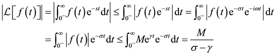(3)

where with real numbers. For example, is not of exponential order. Such functions with extremely fast growth are ignored as economic variables, but there would be no problem in practice.

We consider the Laplace transform of derivatives. Suppose that are continuous on and of exponential order and that is piecewise continuous on and of exponential order. Then

(4)

We obtain with initial condition. Each initial value is considered as left-hand limit at the origin. Suppose that exists. Consider . From the left-hand side, we have

Then, it follows that

(5)

with initial condition. This is called the final value theorem.

Let us consider the Laplace transform of integrals. Let be piecewise continuous on and of exponential order. Putting, we have

(6)

We obtain the Laplace transform of constants as follows:

(7)

We define a transfer function of economic variables. Let economic variables and be of exponential order. Consider the following linear ordinary differential equation with constant coefficients:

(8)

Suppose that and are continuous on and of exponential order and that and are piecewise continuous on and of exponential order. It follows from (4) that

(9)

with initial conditions and. The ratio of the Laplace transforms is called the transfer function. We assume that all the economic variables are of exponential order and that the above continuities and initial conditions hold to obtain the form of (9).

3. The Model

The Phillips’s multiplier-accelerator model is described by

(10)

where aggregate economic variables, , , , , denote demand, production, consumption, investment, autonomous demand, and government spending, respectively. These values can be negative on because they represent the deviations from the levels at. l is a positive constant representing the marginal leakage. The positive constants denote the response speeds in production lag and investment lag, respectively. Since the time unit can be taken arbitrarily, we suppose.

The desired production level is taken as a reference, , and hence denotes the deviation between current and desired level of aggregate production. We suppose that the same equilibrium level is held in, i.e.,

(11)

The exogenous constant deviation in autonomous demand over is written as

(12)

where A is a bounded constant. Clearly the initial values are 0, i.e.,.

If such an exogenous change in autonomous demand occurs, the equilibrium level of aggregate production will shift to another level, involving cyclical fluctuations. Thus, Phillips proposed a policy function for government spending as follows:

(13)

where are positive constants. The target of stabilization policy is to achieve the asymptotic stability. In this process, cyclical fluctuations are preferably suppressed.

The policy lag until demand is affected is supposed as

(14)

where is a positive constant representing the response speed of policy lag.

Taking the Laplace transform of (10), (13), (14), we obtain³

(16)

Thus, the transfer function of and is given by

(17)

We assumed that and are continuous on and of exponential order and that and are piecewise continuous on and of exponential order⁴. Here, all the initial values are 0.

4. Shift of Equilibrium Level

We should qualitatively verify the capability of Phillips-type policy to achieve the asymptotic stability of original equilibrium level. First, we see the effect of exogenous change in without policy.

Theorem 1. An exogenous change in shifts the equilibrium level of production from 0 to A/l.

Proof. Put in (16). We have

(19)

Thus, it follows from (5), (7), (19) that

(20)

W

Next, we analyze the effects of both the proportional and derivative policies,.

Theorem 2. For, the proportional policy can recover the equilibrium level to. The derivative policy does not affect the equilibrium level.

Proof. Put in (17). We have

(21)

Thus, it follows from (5), (7), (21) that

(22)

The terms originate from the derivative policy. Since they converge to 0 as, the derivative policy does not affect the equilibrium level. The derivative policy is used in order only to suppress cyclical fluctuations. W

Finally, we confirm the asymptotic stability by using the integral policy.

Theorem 3. For, the Phillips-type policy (13) can recover the equilibrium level to 0.

Proof. It follows from (5), (7), (17) that

(23)

W

5. Stability Condition

Notice that since the final value theorem can be used when exists, the time path is not ensured to be stable. Various combinations of policy parameters can be taken to achieve the stability, but the parameter constraints are not clear. We therefore focus on the condition on policy parameters to ensure the stability. As is well-known in control theory, the necessary and sufficient condition of asymptotic stability is that all roots of the denominator of transfer function have negative real parts⁵.

Theorem 4. The necessary and sufficient condition for asymptotic stability of the multiplier-accelerator economy with policy (16) is as follows:

(24)

and all the leading principal minors of a matrix

(25)

are positive.

Proof. The Routh-Hurwitz theorem⁶ gives the necessary and sufficient condition for all the roots of a nth- degree polynomial

(26)

with real coefficients to have negative real parts. The condition is as follows: the coefficients exist and have the same sign. In addition, all the leading principal minors of the Hurwitz matrix

(27)

are positive. We can apply the Routh-Hurwitz theorem to the denominator polynomial of (17). From definition, we obtain. Similarly, the coefficients must have the same sign. Namely, and must be satisfied. Moreover, the matrix (25) is the corresponding Hurwitz matrix. W

6. Conclusion

We have established a novel analytic framework on Phillips’s stabilization problem by using the Laplace transform method. On the basis of this formulation, the effects of Phillips-type policy on equilibrium level have been analyzed rigorously and qualitatively. Furthermore, we have derived the stability condition of the model by using the Hurwitz theorem. The present study has shown that the Laplace transform approach is powerful to analyze the stabilization problem. This method will give a fresh insight into the problem on stabilization policy design.

NOTES

¹Some later work used the Laplace transform only to solve the differential equations of the Phillips model [5] [6] .

²See e.g., [5] [7] .

³As shown in (16), the Phillips’s notation with differential operator D is justified by the Laplace transform. For instance, Phillips wrote the production lag as

(15)

⁴It is easy to see that (16) corresponds to the following differential equation:

(18)

⁵See e.g., [8] .

⁶See e.g., [9] and mathematical appendix B in [10] .

Conflicts of Interest

The authors declare no conflicts of interest.

References

[1]	Phillips, A.W. (1954) Stabilisation Policy in a Closed Economy. The Economic Journal, 64, 290-323. http://dx.doi.org/10.2307/2226835
[2]	Hansen, L. and Sargent, T. (2008) Robustness. Princeton University Press, Princeton.
[3]	Bromwich, T.I. (1917) Normal Coordinates in Dynamical Systems. Proceedings of the London Mathematical Society, 2, 401-448. http://dx.doi.org/10.1112/plms/s2-15.1.401
[4]	Carson, J. (1926) The Heaviside Operational Calculus. Bulletin of the American Mathematical Society, 32, 43-68. http://dx.doi.org/10.1090/S0002-9904-1926-04162-8
[5]	Allen, R.G.D. (1966) Mathematical Economics. Macmillan, London.
[6]	Allen, R.G.D. (1967) Macroeconomic Theory: A Mathematical Treatment. Macmillan, London.
[7]	Kreyszig, E. (2011) Advanced Engineering Mathematics. Wiley.
[8]	Bakshi, U.A. and Bakshi, V.U. (2010) Control Systems. Technical Publications.
[9]	Gantmacher, F. (1959) The Theory of Matrices. Chelsea, New York.
[10]	Samuelson, P.A. (1947) Foundations of Economic Analysis. Harvard University Press, Cambridge.