Influential Factors in the Econometric Modeling of the Price of Wheat in the United States of America ()
1. Introduction
Wheat is the most important agricultural commodity in the United States and is considered, to be the principal cereal grain, grown in nearly every state [1] . The US ranked 3rd in production volume of wheat, behind India and China, producing over 3021 million bushels (1 bushel dry volume imperial measure used in the US approximates to 35.2 metric liters/equating to 27.2 kg of wheat at 13.5% moisture content), close to 55.1 million tons, during the 2013/2014 marketing season. The US marketing season for wheat runs from June to May of the next year) [2] . There are over 8 main varieties of wheat grown in the United States, Hard Red Winter Wheat (HRW) makes up 40% of the production, grown across the US between latitudes between 30˚ (Texas) to 49˚ (Montana/Canadian border) [1] . Wheat is a major contributor to the agricultural sector with uses in many areas; such as human food production, beverages, textiles, animal feed etc. All such categories of commodity require wheat inputs and contribute to the immense economic value to the US economy [3] .
The 2008 financial crisis affected the entire globe, causing a sharp spike in the price of wheat and other agricultural commodities [4] . This crisis not only affected those in the developing world but also in economically developed countries such as the US, causing a severe tightening of household budgets in real terms. While the 2008 financial problems focused the attention on the price of commodities, according to macroeconomists, food commodity prices in general have, in fact, been unpredictable since the mid-1990s [4] . Therefore, as the importance of wheat increases, the need to understand and explain the variation in the price of wheat becomes very important.
A wide range of sources of literature provide useful information in regard to the determination of the price of wheat. These include supply factors, demand factors, stock factors, economic factors, and additional commodities prices influencing the wheat price. These different factors integrate a large volume of different data interactions to create mathematical functions or operators which interact with each other as regressors to calculate the price of wheat [4] - [6] . An explanation of these factors will be provided below (Description of Variables). The unpredictability of the price of wheat allows for the creation of a problem to be investigated using research methods. The problem, in its simplest form can be stated as follows:
- To what extent can the variation in the price of wheat within the United States (US Dollar per bushel), be explained by a combination of economically related functions, created by an array of variables related to the US economy?
Secondary to this problem is the question:
- What are the probable causes of the unexplained variation, not related to random error within the wheat price model?
Thirdly:
- Do any weather related regressors influence the variation in the price of wheat at a statistically significant level?
The research questions stated above justify the general hypotheses of this investigation:
Ho: There is a statistically significant relationship between the yearly average price of HRW wheat and supply, demand, macroeconomic, climate and natural resource related functions and the variation within the price of HRW can be explained to an economically acceptable degree.
Ha: There is no statistically significant relationship between the yearly average price of HRW wheat and supply, demand, macroeconomic, climate and resource related functions and the variation within the price of HRW is not accounted for by said functions.
2. Description of Variables, Model and Method/Techniques
2.1. Data Variables/General Description of the Data Used in the Analysis
The dependent variable in question is the price of wheat (Hard Red Winter, for reasons explained in the Introduction) and is in the form of the yearly average price (US$) within the US agricultural marketing season. The data series of the dependent variable dates from the year 1970 to the year 2014, giving a 45-year data set (N = 45) of individual yearly prices given to the nearest cent (i.e. US$ to two decimal places). The source of this data is the United States Department of Agriculture―National Agricultural Statistics Service [2] and has been independently verified by the International Monetary Fund (IFM) and the Food and Agriculture Organization (FAO). The data (both in list and graphical form) of this dependent variable and independent variables analyzed in this investigation can be found in the Statistical Appendix.
To determine what is required for each function used in the creation of a model, an extensive data mining mission was undertaken. The mining of “big data” is the practice of examining a large database in order to generate new information. In total over 1336 different variables were examined [7] in a pre-modeling process to best identify the required variables used to create separate functions, in an attempt to find a best fit model for the intended dependent variable.
To find a suitable model, with an acceptable explanatory power the general agricultural commodity formula of price prediction is:
Equation 1.
Price = constant (β0) + “supply function”*(β1) + “demand function”*(β2) + “macroeconomic function”*(β3) + “natural resource function”*(β4) + “climate function”*(β5)
- Climate function included for research purposes
The “supply function” in simple terms is determined by the amount of acreage harvested for the grain and the yield in bushels. This figure is calculated by multiplying the number of kernels per head of the crop by the number of heads in 3ft by 0.0319 [8] . This formula provides a yearly supply figure in bushels against area, integral in the creation of an agricultural price commodity model [8] .
The “demand function” consists of an integration of components of the supply function and market demand. Widely used within other price commodity models, the Stocks-to-Use ratio indicates the level of carryover stock for a given commodity as a percentage of the total demand. The Stocks-to-use Ratio is simply calculated by: The market season beginning stock level + total yearly production ? total use divided by the total use, then multiplied by 100 to gain a Stocks-to-Use % [6] . As the demand function consists of parts of the supply function, the issue of multi-collinearity within a model may arise; therefore techniques to remove multi-collinearity must be implemented when creating the final model.
The “macroeconomic function” within the model is derived from a calculation of the US yearly average inflation percentage inferred from the Consumer Price Index. Previous research, such as the work of Furlong and Ingenito [9] indicate a relationship between agricultural commodity prices and inflation is present, therefore using inflation as a macroeconomic function could be statistically significant, as a previous relationship has been established in other literature.
The price of crude oil has been previously cited has a weight influencing regressors in the price of agricultural commodity prices. Oil (in the form of petrol and diesel) is an agricultural production input, used in the production of fertilizer, mechanical fuel and transportation, therefore changes in the price of oil will subsequently influence the production of grain commodities and therefore commodity price [10] . The price of oil is referenced by “West Texas Intermediate (WTI-Cushing). WTI, a crude stream produced in Texas and southern Oklahoma which serves as a reference or “marker” for pricing a number of other crude streams and which is traded in the domestic spot market at Cushing, Oklahoma. WTI Crude Oil price per barrel yearly average has been designated as the “natural resource function”, as oil has the biggest influence over agricultural commodity prices in comparison to other natural resources [11] .
As indicated by the third section of the Problem Statement, research by Keatinge et al. [12] and Keatinge et al. [13] indicates that long term temperature records have implications for commodity production worldwide. Therefore as an added measure, the ENSO related Oceanic Nino Index yearly average will be tested for significance within the crop price model as a “climate function”. Therefore to summarize the information about the dependent and independent variables, calculated from the various functions and operators are as follows:
Dependent variable (Y):
- US$ HRW wheat per bushel
Independent variables (X):
- Wheat yield of bushels per acre (BPA).
- US stocks-to-use ratio (STU).
- US yearly average inflation rate (AIR).
- The price of crude oil per barrel (WTI-Cushing) adjusted for inflation (COB).
- ENSO related Oceanic Nino Index (ONI).
2.2. Model and Techniques
The nonparametric correlations of the dependent variable and independent variables were assessed to understand the primary relationships. The results show that both the price of crude oil per barrel adjusted for inflation and the yield of bushels of wheat per acre had a moderately strong positive relationship, whereas the Stocks-to-use ratio exhibited a strong negative relationship, with these three variables correlation was significant at the 95% confidence level (2-tailed). The US inflation rate and the ENSO index showed small negative correlations but were not flagged as significant at the 95% confidence level (see Statistical Appendix for tabled results).
Ordinary Least Squares (OLS) regression was implemented to establish the relationship between the variables to create an acceptable model to predict the price of HWR wheat. The first model created using regression analysis was conducted without considering the interaction among the regressors, using the enter method for the variables (all independent variables were included in the equation in one step). Surprisingly, the model resulted in an F value equating to 51.172, indicating that the regression model has good explanatory ability (51.172 > F (0.05, 5, 39 degrees of freedom) = 2.46). The F statistic is further validated by the R2 value of 0.868 and adjusted R2 of 0.851, indicating that the variables explain 85% of the variation within the dependent variable. Furthermore, all independent variables pass the t-test at the 95% confidence level, meaning that all independent variables have some influence on the dependent variable at the 95% confidence level. Additionally to this, the Durban Watson (DW) Statistic returned a value of 1.808 (close to 2.000). The bounds of the DW at a 95% confidence level where N = 45 and K’ = 5, dL = 1.287 and dU = 1.776. DW value 1.808 > DW upper (dU) are 1.776, therefore we fail to reject the null hypothesis of zero autocorrelation in the residuals, indicating multi- collinearity does not exist among the variables. The initial model (Model 1) can be displayed as:
Equation 2.
(1) 
This model may be further improved by two methods, considering the interaction between variables and the introduction of time as a variable. As the dependent variable is linear in time we can introduce a successive variable indicating the year. The 5 independent variables and time were data-mined to create as many interactions as possible between the variables and transformations of the variables themselves (natural logs, squaring, cubing etc.) in an attempt to improve the explanatory power of the model in comparison to Model 1. An additional method to improve the model is the change in the way the variables are introduced into the model. After the extensive data mining procedure and assessing a variety of different methods of entering the variables the statistical software found that the forward stepwise procedure produce the best model (Model 2), with the following independent variable interactions:
Equation 3.
(2) 
To clarify, Model 2 contains the variable interactions:
- Bushels per acre * Crude oil per barrel.
- The Natural Log of the Stocks-to-use ratio.
- Bushels per acre * Yearly average inflation rate.
- Crude oil per barrel * Oceanic Nino Index
- Date in the form of the year.
- Oceanic Nino Index * Oceanic Nino Index
Model 2 provided an improvement on Model 1, the model resulted in an F value of 60.068, increasing the explanatory power (60.068 > F (0.05, 7, 37 degrees of freedom) = 2.275). The model had an improved R2 of 0.919 and an adjusted R2 of 0.904, all variable interactions passed the t-test at the 95% significance level, indicating they all have an influential power within the model. Model 2 also improved on the Durban Watson Statistic with a value of 2.132 (close to 2.000). The result of 2.132 > DW upper (dU) 1.895 means we fail to reject the null hypothesis of zero autocorrelation in the residuals, implying there is no evidence of positive first-order serial correlation of residual series, see Tables 1-3 and Figure 1 and Figure 2 for a summary of results.
2.3. Theoretical Justification of the Model
To provide theoretical justification of the model we must perform two actions, firstly a comparison of the two models stated to statistically prove which model is better and secondly to validate the assumptions of Ordinary
![]()
Table 1. Tables displaying the results of the regression analysis of Model 2.
Durbin-Watson = 2.132.
![]()
Table 2. Analysis of variance (ANOVA) of Model 2.
aPredictors: (constant), Bushels_Crudeoil, Ln_stockstouse, Bushels_Inflation, Crudeoil_ENSO, Yeild_Bushel, Year, ENSO_Squared.
![]()
Table 3. Atable displaying the model coefficients.
Least Squares regression modeling.
To find the best model two comparison methods were introduced, the Corrected Akaike’s Information Criteria (AIC) of both models were compared and an F-test was performed. Model 1 had a Sum-of-squares of 19.078, N = 45, Parameters = 5 resulting in a correct AIC of −24.41. Model 2 has a Sum-of-squares of 11.66, N = 45, Parameters = 7 resulting in a corrected AIC of −40.77. These results indicate that Model 2 has a lower AIC than Model 1, indicating that Model 2 has a better performance ratio than Model 1.
Additionally, the F-test was performed on the models as a secondary comparison method. As mentioned above, Model 1 has a Sum-of-squares of 19.078, 40 degrees of freedom; Model 2 has a Sum-of-squares of 11.66, 38 degrees of freedom resulting in a percentage difference of 63.62 and an F value of 12.087.
![]()
Figure 1. A normal P-P plot of the standardized residual of the depended variable displaying the expected cumulative probability against the observed cumulative probability.
![]()
Figure 2. A scatterplot of the actual price of wheat per bushel against the regression adjusted predicted value.
Equation 4.

Equation 5.

Since the F value > F statistic we can say there is statistical evidence to suggest that Model 2 performs better than Model 1, according to both the reduction in the AIC and the results of the F-test.
We must also provide validation that the model created meets the assumptions of OLS regression (normally distributed error, independent error structure, homoscedastic error and zero covariance of error within the predicted values). Firstly we must examine the errors terms as a result of the regression model, i.e. the mean of the value of the error terms should be equal to zero, the residuals should be distributed symmetrically about the expected values and that the error terms follow a “normal” distribution.
The results indicate that the residuals pass the first two criteria but fail on the third (the mean of unstandardized residuals = 0 and are distributed symmetrically about the mean―see Statistical Appendix). Testing for normality reveals that the errors terms are not normally distributed and the model fails the assumptions of OLS. The tests for normality show the model passing the Kolmogorov-Smirnov test but failing the Shapiro-Wilk test. The results indicate that two observations skew the distribution and are considered outliers, observations 2007 and 2012; this is also confirmed by the Cooks Distance values of these observations (2007 = 0.2878 and 2012 = 0.126386). Upon removal of these cases and retesting we find that the error terms mean the assumption of normality passing both the Kolmogorov-Smirnov test and Shapiro-Wilk test, therefore validating the assumptions of OLS regression.
Another assumption of OLS regression is that the error series is independent of Y and the regressors. The results indicate that this assumption is met with all covariance values for the error and variable series equaling zero (see Statistical Appendix for full results).
Equation 6.

The last assumption of OLS regression is the variance in the distribution of stochastic error is homoscedastic. The results indicate that the error is indeed homoscedastic, as shown by the horizontal fit-line of the scatterplot of the standardized residual against the standardized predicted value (Statistical Appendix). The results above confirm that the best model selected meets the assumptions of OLS and provides theoretical justification of the model.
3. Interpretation/Summary of Results
As the results from the previous two sections indicate, the model created is generally a good fit-for-purpose, given the amount of variables/interactions and use of “natural data” when explaining the variation in the price of wheat. The figure below (Figure 3) displays the actual price of wheat per bushel against the model predicted price of wheat per bushel. The results indicate that some areas of the model provide better results than others, for example, the model indicates a cyclic variation through 1980-1986 whereas the real data indicates a general decline in wheat price. The results also indicate that the model is sensitive to the prediction of extreme price drops (negative price spikes), such as in 1975 and 1998, but not as sensitive to the prediction of extreme price increases (positive price spikes) as in 2007 and 2012. This may suggest that there are further factors that influence the price of wheat in addition to the functions (regressors) stated in the variable description section. This observation will be further discussed below (Discussion of Relevant Findings section).
To summarize, the OLS regression analysis, taking into account variable interaction, provided a satisfactory model to establish a relationship between “supply”, “demand”, “macroeconomic”, “climate” and “natural resource” related functions to explain the variation in the price of wheat. The model returned an F-value of 60.068 and an R2 of 0.919/adjusted R2 of 0.904. upon removal of outliers the model met the assumptions of OLS regression providing theoretical justification of the model and Model 2 was statistically proven to be the best model (lowest AIC and F-test results). But with an adjusted R2 of 0.904 nearly 10% of the variance within the price of wheat remains to be explained. The section below discusses this issue and attempts to explain the remaining variation
![]()
Figure 3. A graph to show the actual price of wheat per bushel against the model predicted price of wheat per bushel in US dollars. The model shows sensitivity to a rapid decrease in the price of wheat (negative price spike). But the model shows a lack of sensitivity to a rapid increase in the price of what (positive price spike). *for discussion purposes relating to speculation and additional economic activity, the observations from 2007 and 2012 have been included in this graph.
that is unexplained by the model.
4. Discussion
The results of this investigation provide an interesting insight into the modeling of the price of wheat within the US. The model, which is generally excellent in its explanatory power, does not account for just less than 10% of the variation within the price of wheat. Therefore we must look for additional factors which may explain this unaccountable variation. Common sense implies two methods of improvement, which are discussed below.
To improve the model stated, adding additional information may provide an explanation of the difference between the real price of wheat and the model predicted price of wheat. Masters [14] addresses the spikes in the price of wheat during the 2007/2008 economic crisis, that are most likely related to the impact of financial speculation and commodity index trading and are not related to real price levels and price volatility in market- specific supply and demand conditions as explained in the model created above. With the 2012 wheat price data also being flagged as an outlier, the cause of this spike may also be related to financial speculation. This idea that financial speculation within the economic markets could provide the reasons for the spikes in price is interesting. As the results show, the model created within this research is sensitive to negative price spikes but insensitive to positive price spikes. Therefore we could speculate that sudden decreases in the price of wheat can be attributed to the functions described in this research, but sudden increases in price may be attributed to speculation within the financial markets [15] .
The reason that the identification of the causes of unpredictable/outlier prices is necessary to implement and evaluate governmental policy (both national and international) in the intervention and adjustment in the price of not only wheat but other related agricultural commodities [16] . Therefore, looking to identify financial speculation on the stock markets as a reason for unpredictable/“un-modelable” price increases is important because governmental intervention can safeguard against artificial price rises. In terms of poverty and food security, being able to predict a rise in price is more important than being able to predict a decrease [17] but the question arises of how financial speculation would be measured and input as a variable into an equation?
Another area where additional information may provide a better model would be increasing and developing the climatic related function within the model. In a similar research project to this (regression modeling the price of soybean in the US), Karthilkeyan and Harlalka [18] returned a similar adjusted R2 value of 0.85 but their model contained far more climatic related regressors than this investigation but fewer macroeconomic and demand factors. Karthilkeyan and Harlalka [18] infer that climatic factors accounted for a substantive variation in the price of soybean in the US, finding both temperature (Fahrenheit) and precipitation (inches) to both be statistically significant in their price prediction model. These additional climatic data sets may be influential in the wheat price model from this investigation but the spatial factors of these data sets pose a tough problem for consideration. Soybean within the US is only grown in relativity small areas compared to wheat (e.g. Mississippi/ Arkansas/Louisiana border and parts of Illinois and Iowa). Measuring the climatic influences on soybean is a much easier task. Due to the widespread areas over which wheat is grown in the US (as stated in the introduction), the range and diversity of climatic conditions within these areas in far greater than that of where soybean is grown.
Another method which may improve modeling capability would be to apply different statistical modeling methods other than OLS regression. Janzen et al. [4] apply a structural vector auto-regression model (SVAR) to identify the influential drivers on the price of wheat (in this case the market futures price of wheat). Similar to the pre-modeling process of this investigation, i.e. the creation of separate functions that create individual variables. Janzen et al. [4] created individual linear models of different variables associated with modeling the price of wheat. In a complicated statistical procedure the SVAR model predicts structural shocks associated with each variable to identify which variable is the underlying cause in both positive and negative price spikes. The authors found that spikes in price are fundamentally driven by supply factors and that current financial problems and unpredictability are not related to financial speculation and commodity index traders. The increase in price during the 2007/2008 period can, according to Janzen et al. [4] , be attributed to Australian drought conditions. But this theory can be disproven by the results of this investigation, as ENSO related SSTs, the driving factor behind El Nino and La Nina weather related phenomenon are a variable within the OLS model created above and it has proven to be statistically significant.
Roache [19] attempts to examine the changes in the price of agricultural commodities by using a spline- GARCH model (a generalized autoregressive conditional heteroscedasticity model integrated where the error variance is assumed to be an autoregressive moving average model (ARMA)) developed by Engle and Rangle [20] . Roache [19] found that the measure of volatility has risen for a range of different commodities during the last 10 years, indicating that the predictive power of price commodity models has become sporadic. As with this research, the author highlights the need for further research into the relationship between agricultural commodity prices and financial speculation, especially the relationship between futures trading volumes and real commodity prices [21] . This point is extremely valid when considering the lack of regulation for speculation on the global futures markets. As the author of this investigation can stress, anyone (regardless of training) can speculate on the futures market, regardless of economic training and education.
5. Conclusions and Future Research
The results of this investigation allow us to firstly answer the problem questions stated in this paper and secondly to “fail to reject” the general hypothesis stated. Therefore to conclude this investigation we can state, in answer to the problem questions stated earlier, that:
- We can explain the variation of the price of wheat within the United States to 90.5% according to statistical evidence based on the OLS regression model of a combination of “supply”, “demand”, “macroeconomic”, “climate” and “natural resource” related functions.
- There could be several causes of the variation within the price of wheat that the model created which have been left unexplained. These range from adding additional data sources, such as adding climatic data and financial speculation data and improving variable interactions to performing different statistical modeling techniques, such as SVAR and Spline-GARCH modeling.
- Lastly, weather related regressors were found to be statistically significant in the contribution to the price of wheat at a 95% confidence level, as shown by the ENSO related ONI interaction within the model.
The results of this investigation and the points raised in the discussion have various implications and inspire ideas for future research. The main implication is that the price of wheat can be modeled to a reasonable accuracy but there are areas in which future research could focus, such as developing methods to measure financial speculation etc. The recreation of this investigation on a monthly scale may be the best course of future action. Further research into the addition of weather related variables would also be an appropriate course of action.
Acknowledgements
Fergus J. D. Keatinge would like to thank the creators of the statistical software package IBM SPSS software, The World Bank for providing the data requires for the analysis and Dr. Timothy Fik of the University of Florida, for his teaching, ideas and suggestions for this research.
Statistical Appendix

Statistical Appendix Figure 1. Raw data.

Statistical Appendix Figure 2. A graphical depiction of the raw data.
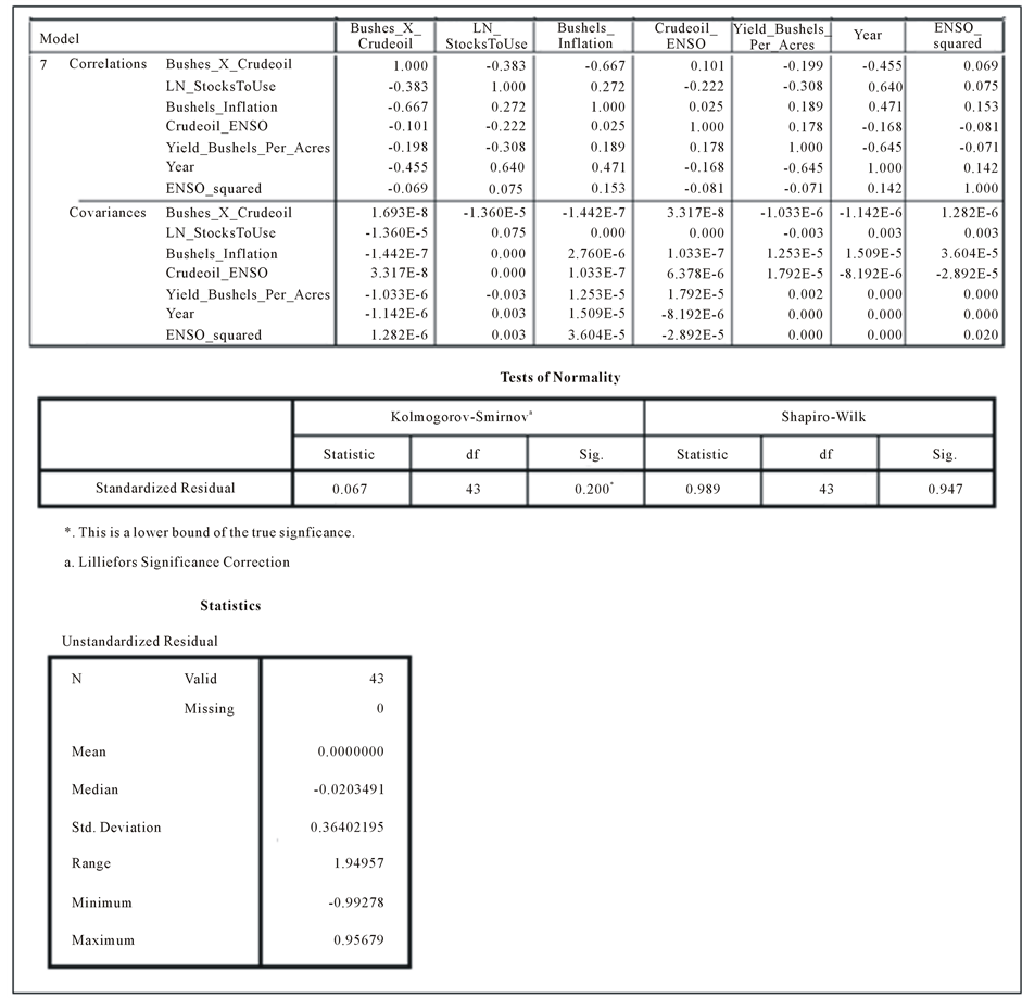
Statistical Appendix Figure 3. Various tables displaying the variable covariances, normality error tests and descriptive statistics of the residuals.
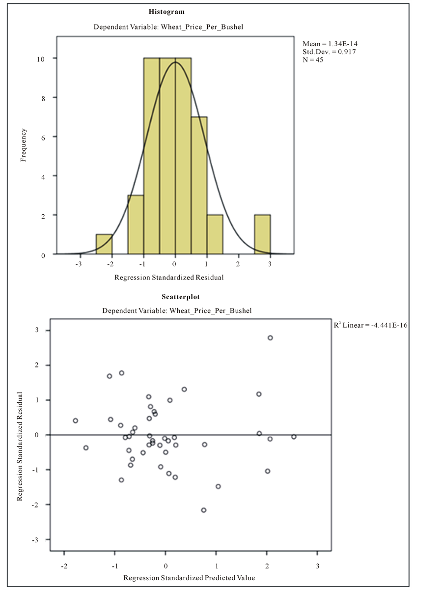
Statistical Appendix Figure 4. Two figures showing the histogram of the frequency of the standardized residuals and a scatter plot of residual against predicted value.