1. Introduction
George Pólya, Hungarian mathematician, observed that when a proof is too simple, “youngsters” will be unimpressed [1] , but mathematics does not have to be complicated to be useful. He also pointed out that solving problems is a quintessential human activity and the aim is always to find the simplest solutions.
Not all scientists are attracted by complicated mathematics but it does not mean that they do not carry out an excellent and important research work. If they could be presented with a simple but useful method of analysis they could apply it productively in their scientific research.
We are going to describe a simple method of analysis of hyperbolic processes. For mathematicians, the explanation of this method might sound too trivial but our aim is to make it available to those who are less skilful in mathematical analysis of data. However, before we offer a solution we have to understand the problem.
2. The Common Problem
Hyperbolic processes appear to be causing an insurmountable problem in certain fields of research. They create such a strong illusion that it deceives even the most experienced and respected researchers. Whether discussed explicitly by displaying the relevant data or implicitly by referring to data associated with such distributions, the common mistake [2] -[74] is to see them as being made of two distinctly different components, slow and fast, with a clear transition between them. The next step is then to try to explain these two perceived stages of growth and the associated but non-existent transition by proposing distinctly different mechanisms for each of these imagined components rather than seeing them as representing a single, monotonically increasing distribution governed by a single mechanism of growth.
This step leads progressively further away from the correct understanding of studied processes because all efforts are now concentrated on explaining the non-existing features. An increasing number of scholars are being involved. They do not analyze the relevant data but only describe their impressions created by hyperbolic illusions. The participating researchers do not question the existence of the distinctly different stages of growth or of the postulated transition—they take them for granted and concentrate their attention only on the explanation of these phantom features, proposing new mechanisms, theories and mathematical descriptions without realizing that the apparent distinctly different two stages of growth do not exist and that there is no transition but a monotonically increasing hyperbolic distribution. Their mathematical descriptions, complicated and elaborate as they might be, are not the descriptions of the studied processes but rather the descriptions of phantom images created by hyperbolic illusions.
The perceived two stages of growth are commonly described as stagnation and sustained growth, while the perceived but non-existent transition as an escape, sprint, sudden spurt, intensification, acceleration, explosion or by some other similar terms all emphasizing a clear and dramatic change in the pattern of growth at a certain time. Variety of forces and mechanisms are then proposed to explain the phantom stages of growth and of the associated but non-existent transition. Efforts are also made to determine the precise time of the non-existent transition, often placing it around the Industrial Revolution but sometimes around 1950, without realizing that the determination of the time is impossible because there was no unusual acceleration at any particular time or over a certain range of time.
Hyperbolic processes are prone to misinterpretations and consequently they have to be analyzed with care. Fortunately, their analysis is exceptionally simple. To show how to avoid being guided by hyperbolic illusions we shall first describe the method of data analysis and then illustrate it by using a few examples.
3. Description of the Method
Hyperbolic processes can be easily analyzed using the method of reciprocal values. This method is so simple that it can be explained by using just two elementary equations, and yet so powerful that it can turn around and revolutionize such fields of research as the economic growth and the growth of human population, the important fields of study because for the first time in human existence we have now reached the ecological limits of our planet and the correct understanding of these two processes is essential to avoid the undesirable unsustainable developments. We have to know how these processes work and how to control them. Incorrect interpretations are potentially dangerous and cannot be tolerated. Every effort has to be made to identify and eliminate any incorrect and misleading explanations.
The first-order hyperbolic distribution is described by the following simple equation:
 , (1)
, (1)
where  is the size of a growing entity, while
  and
and  are constants. For the hyperbolic growth,
 .
.
An example of a hyperbolic growth is shown in Figure 1. Such a growth can be easily seen as being made of two components, slow and fast and that is why the misinterpretations of hyperbolic processes are so common and the need for a simple method of their analysis so urgent, a method that can be understood and used by anyone. The distribution presented in Figure 1 was generated by fitting the growth of the world population. The parameters describing this distribution are  and
and .
.
It is certainly true that the growth shown in Figure 1 was slow over a long time and fast over a short time. These features are undeniable. The mistake does not consist in seeing them for what they are but in their interpretation.
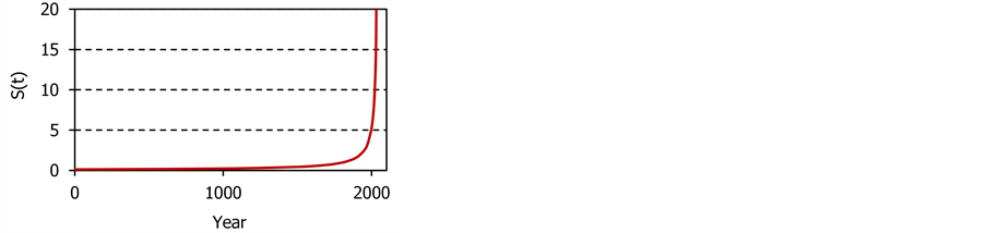
Figure 1. An example of a hyperbolic growth.
It is incorrect to interpret such a growth as being made of two distinctly different components prompted by two distinctly different mechanisms. It is precisely at this junction that a serious mistake is commonly made and the research is diverted into pathways that lead progressively further away from correct interpretations of hyperbolic processes, the pathway leading from science to fiction.
The apparent slow and the apparent fast components belong to the same hyperbolic distribution and are governed by the same mechanism of growth. There is no separation between them. However, the illusion of the existence of two components is so strong that it generates endless discussions in the economic and demographic research and leads to many intricate and complicated but incorrect and misleading explanations of growth. The illusion readily disappears when we display the reciprocal values of data because in this representation the hyperbolic growth is shown as a simple and an unambiguous straight line:
 . (2)
. (2)
The reciprocal values of the growth presented in Figure 1 are shown in Figure 2. What might have looked like a distribution made of two or maybe even three components in Figure 1 is now clearly shown as a distribution made of just one component. The hyperbolic illusion interfering with the correct interpretation of growth is replaced by a simple pattern, which is easy to understand and interpret.
Properties of growth do not change by changing the display of data but certain features, which are difficult or even impossible to recognize in one display can be easily identified in another. When the reciprocal values of data are displayed, the deviation to a slower trajectory will be indicated by an upward bending and the deviation to a faster trajectory by a downward bending.
When hyperbolic growth is represented by a mathematically generated and gradually changing curve, such as shown in Figure 1, it might be clear that there was no particular time when the growth changed from being nearly horizontal to nearly vertical, but when data represented by discrete points are displayed, such a conclusion might be less obvious. The illusion becomes particularly strong when only a few strategically located points are selected [2] [14] -[22] [25] [74] from a significantly larger set of data as if to make the deception even more pronounced. Even if the enforcement of the perceived illusion is unintended, such crude displays of data lead readily to grossly incorrect interpretations.
However, if the reciprocal values of data are displayed, their analysis is immediately made significantly simpler because if the data follow a simple, first-order hyperbolic distribution, their reciprocal values will be clearly aligned along a decreasing straight line. It is then obvious that dividing such a straight line into two sections and claiming two distinctly different regimes of growth governed by two distinctly different mechanisms simply makes no sense. It makes also no sense to try to locate a point on the decreasing straight line and claim a transition between two arbitrarily chosen sections.
It should be stressed that in this representation only the first-order hyperbolic distributions describing growth will follow the decreasing straight line trajectories. It is for this reason that this simple method is so useful in identifying the first-order hyperbolic distributions. It is a simple and yet powerful method, which can be used successfully in the analysis of data describing the historical economic growth and the growth of human population, global, regional or local, because in general they follow simple, first-order hyperbolic trajectories. Any deviations from such trajectories can be easily investigated. Higher-order hyperbolic distributions describing growth will be represented by gradually decreasing trajectories, which could be fitted using higher-order polynomial functions intercepting the horizontal axis, while the exponential growth will be represented by a decreasing exponential function.
This method might have a more general application but its specifically intended application described in this publication is to help to avoid being guided by hyperbolic illusions, the unfortunate common mistake, which often leads to seriously incorrect conclusions as we shall demonstrate in the examples 2 and 3.
Going beyond the intended application, the first-order decreasing hyperbolic distributions will be represented by the increasing straight lines. Again, in this representation, any deviation from the decreasing hyperbolic distributions can be easily detected and investigated. The Pareto distributions that look like hyperbolic distributions will be represented by gradually increasing functions, which in this representation might be also easier to investigate.
We shall now illustrate the application of this method by using three examples: the growth of human population in Africa, the economic growth in Western Europe and the examination of the fundamental postulates of the Unified Growth Theory [14] [20] .
4. Examples
4.1. Example 1: Population Growth in Africa
The method of reciprocal values can be used to study fine details of growth trajectories, the study which can then be used not only to improve the fit to the data but also to understand the mechanism of growth. Some distributions, which appear to be hyperbolic, might be made of different components. Such components might be difficult or even impossible to see in the direct display of data but they can be easily revealed by displaying their reciprocal values. An excellent example is the growth of human population in Africa shown in Figure 3, constructed using Maddison’s data [75] .
The top panel in Figure 3 contains the direct display of data for the growth of human population in Africa. The displayed shape suggests hyperbolic growth, but the lower panel, which shows the reciprocal values of the population data, reveals that the hyperbolic-like growth trajectory is in fact made of two major components, slow and fast. However, it shows also that the slow component does not represent a stagnant and chaotic state but a steadily increasing hyperbolic growth. The parameters describing the two hyperbolic components are ,
,  for the slow component and
 ,
,  for the fast component.
Furthermore, the transition, which is impossible to identify in the top panel, is now clearly seen in the lower panel. The transition occurred around 1870 but it was not a transition from a stagnant growth to a distinctly different “sustained growth”, but from a sustained slowhyperbolic growth to a sustained fasthyperbolic growth.
Not only can we now see clearly the change in the pace of growth but also we can determine fairly precisely the time of the unusual acceleration. We can also study closely the character of the two trajectories, before and after 1870. We can see clearly that both of them were not only hyperbolic but also that they followed the simplest, first-order, hyperbolic distributions.
The data show also that from around 1975 the growth trajectory of the reciprocal values started to bend upwards, away from the fast hyperbolic trend to a slower trajectory. Thus, the diversion to a slower pathway, which was impossible to see in the top panel, is now clearly displayed when we use the reciprocal values of data particularly if we magnify the display in this region.

Figure 3. The growth of human population in Africa [75] illustrates how the method of reciprocal values can serve as an excellent tool in revealing hidden features of studied distributions.
So now, the details of the mechanism of growth, which were impossible to identify by the direct display of data, are clearly demonstrated by the reciprocal values. The growth of the populations in Africa was following a slow hyperbolic trend until around 1870. Around that year, the growth of human population in Africa experienced an unprecedented 4-fold acceleration, which diverted the growth into a significantly faster hyperbolic trajectory. The fast hyperbolic growth continued until around 1975 when it started to be diverted to a new but slower trend. Armed with all this useful information we can now try to explain the mechanism of growth in Africa, but such an explanation is outside the scope of this publication.
The reciprocal values of the data after 1975 are not fitted by the straight line but this is precisely where the advantage of this method is so well illustrated. It allows not only for an unambiguous identification of the first-order hyperbolic distributions but also for a clear demonstration of a departure from such distributions.
4.2. Example 2: Economic Growth in Western Europe
Economic growth is measured using the Gross Domestic Product (GDP) or the GDP per capita (GDP/cap). Galor and Moav [25] studied economic growth in Western Europe using the data of Maddison [76] . They have selected four, strategically located points from a larger set of data, joined them by straight lines and concluded that there were two distinctly different regimes of growth: the “Malthusian regime” (also labelled as the “epoch of stagnation”, “Malthusian era”, “Malthusian epoch”, “Malthusian steady-state equilibrium”, “Malthusian stagnation” or “Malthusian trap”) and the “sustained economic growth” (described also as the “Modern Growth Regime”, “sustained economic growth” and “sustained growth regime”). Referring to their crude display of data they also concluded that the Industrial Revolution had a strong impact on the economic growth causing a dramatic takeoff from stagnation to a fast growth. They made no attempt to analyze mathematically Maddison’s data [76] but presented complicated mathematical descriptions of the impressions created by hyperbolic illusions. We shall now use the same source of data to demonstrate that their claims are scientifically unsustainable.
Figure 4 presents the reciprocal values of the Gross Domestic Product (GDP) for Western Europe [76] in the vicinity of the alleged takeoff. The data are well aligned along a decreasing straight line, which means that the GDP was not only increasing hyperbolically but also that it was following the simplest, first-order, hyperbolic

Figure 4. Reciprocal values of thedata descrtibing theGross Domestic Product (GDP) in Western Europe [76] in the vicinity of the Industrial Revolution. The GDP is in billions of the 1990 International Geary-Khamis dollars. Contrary to the claim made by Galor and Moav [25] , the Industrial Revolution had no effect on the economic growth in Western Europe, the cradle of this revolution, and the two regimes of growth did not exist.
distribution.
The Industrial Revolution occurred between 1760 and 1840 [77] , or around 1800 as shown in Figure 4. This figure demonstrates clearly and convincingly that the claimed takeoff around the time of the Industrial Revolution did not happen because the reciprocal values of the GDP data follow an undisturbed straight line trajectory representing an undisturbed hyperbolic growth. It is now clear that there was no takeoff and no escape, great or small, from the hypothetical but non-existing Malthusian trap. The Industrial Revolution had absolutely no impact on the economic growth in Western Europe, the cradle of this revolution. Any explanation of the economic growth as being influenced by this event is not only irrelevant but also incorrect and strongly misleading.
The absence of a takeoff eliminates also the need for assuming the existence of two distinctly different regimes of growth. It obviously makes no sense to divide the straight line into two arbitrarily selected sections and claim distinctly different trajectories governed by distinctly different mechanisms of growth. What might not have been clear in the direct display of data is perfectly obvious if we display the reciprocal values of data. This display abolishes all elaborate theories and explanations incorporating such concepts as traps, escapes, takeoffs and stagnation and replaces them by a simple interpretation of the mechanism of growth in agreement with the general observation that natural phenomena can be usually explained by using simple descriptions.
In Figure 5, the hyperbolic trend corresponding to the straight line shown in Figure 4 is extended to AD 1. There are no economic growth data beyond this point. The economic growth in Western Europe is well described by a simple, first-order, hyperbolic distribution. The corresponding parameters are:  and
and . The point at 1950 is not fitted by the hyperbolic trend because from the early 1900s the economic growth in Western Europe started to be diverted to a slower trajectory.
We cannot claim that the growth was sustained only after the Industrial Revolution because it was sustained equally strongly during the postulated but non-existent “epoch of stagnation”. Figure 4 and Figure 5 show clearly that the concept of two stages of growth is unsupported by data. When stripped of the hyperbolic illusions, the economic growth is revealed as a simple process, which can be described using just one, simple mathematical trajectory. There is no compelling need to make this simple description complicated.
The growth of the GDP was slow in the past because it was hyperbolic. However, while being slow it was not stagnant. The growth was fast in recent years because it was hyperbolic. It followed the same undisturbed hyperbolic distribution as in the past.

Figure 5. The data for the Gross Domestic Product (GDP) in Western Europe [76] compared with the hyperbolic distribution. The GDP is in billions of the 1990 International Geary-Khamis dollars.
We now have a completely different understanding of the economic growth in Western Europe, an important turnaround in the economic growth research. Rather than wasting the valuable time, energy and financial resources on trying to explain the phantom features created by hyperbolic illusions magnified by the customary crude representation of data [2] [14] -[22] [25] [74] we can now focus our attention on the relevant task of trying to explain why the economic growth was so stable over such a long time. Rather than writing numerous articles based on impressions and publishing them in peer-reviewed scientific journals and in academic books we can now concentrate our attention on the understanding the science of the economic growth.
4.3. Example 3: Unified Growth Theory
As a third example of the application of the method of reciprocal values we shall now use Galor’s Unified Growth Theory [14] [20] representing the culmination of his work extending over 20 years [78] . The fundamental postulate of this theory is the existence of three regimes of growth: the slow and stagnant Malthusian Regime, the short and intermediary Post-Malthusian Regime and the fast Sustained Growth Regime. Galor also postulates that the Industrial Revolution played a crucial role in the alleged dramatic takeoff from a prolonged stagnation into a rapid and sustained growth. Maddison’s data [76] are referred to and used to justify the formulation of this theory but no attempt is made to analyze them mathematically. We shall now use exactly the same source of data and show that the Unified Growth Theory is scientifically unstainable.
The reciprocal values of the data for the world Gross Domestic Product (GDP) [76] are shown in Figure 6. They follow closely a decreasing straight line, which means that the economic growth was increasing hyperbolically. It is clear that there was no takeoff of any kind, large or small, around the time of the Industrial Revolution and no repeatedly claimed great escape from the postulated but non-existing Malthusian trap. The data do not support the existence of the three regimes of growth and thus contradict the fundamental postulates of the Unified Growth Theory.
The last point of the data shown in Figure 6 is not fitted by the straight line, suggesting a possible diversion to a slower trajectory. This region can be studied more closely using the extended compilation of the economic growth data [75] . Their reciprocal values between 1700 and 2003 are shown in Figure 7 demonstrating clearly that while the Unified Growth Theory claims an unusually accelerated growth after the alleged but non-existent epoch of stagnation, the data show the opposite behavior: a diversion to a slower trajectory after the earlier vigorous, well-sustained and secure economic growth. Rather than being boosted by the Industrial Revolution, the economic growth continued along the undisturbed hyperbolic trajectory for about one hundred years and then started to slow down.
Figure 7 illustrates again how the method of reciprocal values can unravel useful details about a studied process. Not only does it help in an unambiguous and easy identification of hyperbolic distributions but also it helps in an easy detection of deviations from such distributions. The world economic growth continues to increase but from the early 1900s it started to be diverted away from the faster accelerating historical hyperbolic trajectory to a slower trend.
The point of the intersection of the reciprocal values with the horizontal axis is the point of singularity when
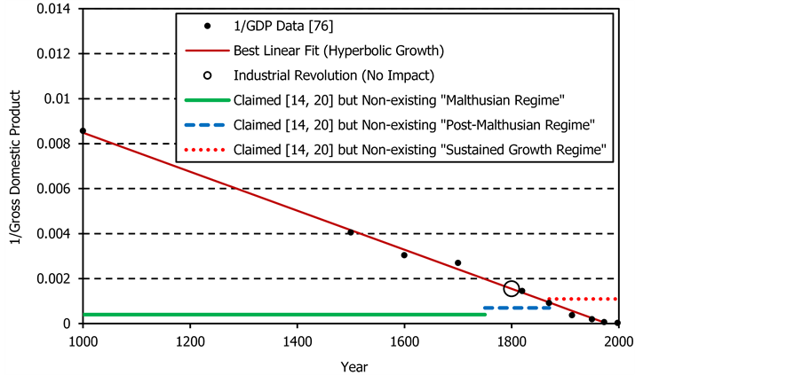
Figure 6. Reciprocal values of the data describingthe world Gross Domestic Product (GDP) [76] and their prevailing linear trend representing hyperbolic growth. The Industrial Revolution had absolutely no influence of the economic growth and the postulated three regimes [14] [18] [20] [22] did not exist.The GDP is in billions of the 1990 International GearyKhamis dollars.
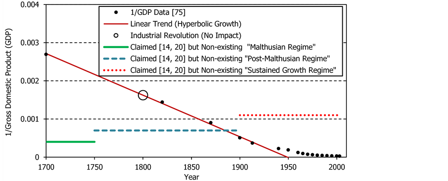
Figure 7. The lower part of Maddison’s data [75] shows clearly that while the Unified Growth Theory [14] [20] [29] [30] claims a vigorous sustained growth after the epoch of stagnation, the data show the opposite behaviour: a diversion to a slower trajectory after the vigorous and secure growth. The claimed [14] [18] [20] [22] [29] [30] but non-existent three regimes of growth are also indicated.The GDP is in billions of the 1990 International Geary-Khamis dollars.
the growth escapes to infinity. No growth can go beyond this point and any growth close to it may become unstable, unsustainable and catastrophic. Figure 6 and Figure 7 show how close we are now to the point of the potential global economic collapse. We have two options: to continue skirting precariously close to the horizontal axis or to try to move away from it by reducing the economic growth.
The Unified Growth Theory claims that after a long time of stagnation we have now reached an era of “sustained economic growth”, the term repeated 82 times in the first detailed formulation of this theory [14] , the potentially misleading description because while it is true that the current economic growth is still sustained the past economic growth was not only sustained but also it was increasing along a more secure trajectory, far away from the point of singularity. Even though the growth became diverted to a slower trajectory any further increase can be potentially dangerous.
The reciprocal values of data show that for the first time during the AD era, and probably for the first time in human existence, we are trapped between the already high level of economic growth and a point of no return, or equivalently between the very small reciprocal values and zero. Any intrusion into this narrow gap has to be closely monitored. Even if the trend of the reciprocal values of the GDP data does not cross the horizontal axis any close approach to this axis could be dangerous, because it could trigger global economic collapse. However, there is also an additional danger that the growth might resume its historically preferable hyperbolic trajectory. Many alternative trajectories could be hopefully controlled to avoid reaching a point of no return but a renewed hyperbolic trajectory so close to the point of singularity would be most likely uncontrollable.
If the economic growth continued along the historical hyperbolic trajectory it would have already reached a point of no return as indicated by the fitted straight line crossing the horizontal axis. To use the colorful description of von Foerster, Mora and Amiot [79] , we have been saved from experiencing a doomsday associated with the global economic collapse. However, the danger of an excessive growth towards the point of no return is still not averted.
Under a suitable control, the economic growth can continue for a long time, but this is precisely the important point: from now on the economic growth has to be closely monitored and controlled. It is essential to understand and accept that the natural tendency of the economic growth, as indicated by the mathematical analysis of data, is to follow a hyperbolic trajectory, which with its current close proximity to the point of singularity could lead to undesirable results. It is also essential to know that the current economic growth is relatively close to the point of no return and consequently that it could become unsustainable.
The data between 1965 and 2003are fitted well by the exponential function  with the doubling time of 20.59 years corresponding to the annual growth rate of 3.37%. The exponential growth will never increase to infinity in a finite time but it also has its limit determined by the availability of resources. Thus, the prolonged exponential growth can also lead to a critical point of no return and to the global economic collapse.
The world GDP in 2003 was $41 trillion  [75] , expressed in the 1990 International Geary-Khamis dollars. If the current exponential growth, as indicated by Maddison’s data [75] , continues undisturbed, it may be expected to reach $1085 trillion in 2100 and $31,452 trillion in 2200. Can such a rapid growth be sustainable?
However, if we assume that the growth will continue along a linear trajectory, i.e. with the hyperbolically decreasing growth rate, then the linear fit to the GDP data between 1995 and 2003 shows that by 2100 the world GDP would increase to only $160.7 trillion and by 2200 to $284.4 trillion, which could be probably manageable. However, the tradeoff is the rapidly decreasing growth rate. By 2100 it would have to decrease to 0.8% and by 2200 to 0.4% per annum. By 2500, the world GDP would increase to $419.8 trillion and the growth rate would decrease to 0.18% per annum. These calculations suggest that a suitably controlled growth between linear and exponential would be probably safe for a long time to come.
If we allow ourselves to be guided by the Unified Growth Theory we might be convinced that after an endless epoch of stagnation we can now enjoy a sustained economic growth. However, if we base our understanding of the economic growth on the mathematical analysis of data we shall realize that the opposite is true: after a steady and secure economic growth in the past we have now reached the stage when we have to be cautious and vigilant. Descriptions based on hyperbolic illusions reinforced by crude representation of data [2] [14] -[22] [25] [74] create a false sense of security while the reality could bring unpleasant surprises. The method of reciprocal values can also be used to demonstrate that two other postulates of the Unified Growth Theory, the postulate of the differential takeoffs and the postulate of the great divergence, while appearing to be supported by the crude representation of data, are contradicted by the mathematical analysis of the same data.
The data describing the world economic growth [76] are compared in Figure 8 with the hyperbolic trajectory calculated using the straight-line fitted to the reciprocal values shown in Figure 6. The parameters describing the historical hyperbolic growth of the world GDP are:  and
and .
.
Now the puzzling features of the economic growth, the features that prompted so many discussions in numerous peer-reviewed scientific journals culminating in the formulation of the Unified Growth Theory, are manifestly clear, and their explanation is surprisingly simple. Over hundreds of years, the world economic growth was slow because it was hyperbolic. Over a short time, until the early 1900s, the economic growth was fast because it was hyperbolic—it followed the same undisturbed hyperbolic trajectory as in the past. The apparent transition from a slow to a fast growth is just an illusion created by the hyperbolic distribution. There was no

Figure 8. The data for the world Gross Domestic Product (GDP) [76] follow closely the first-order hyperbolic distribution. The claimed three regimes of growth [14] [20] are now revealed as an uninterrupted hyperbolic growth.The GDP is in billions of the 1990 International Geary-Khamis dollars.
unusually accelerated transition from the slow to the fast economic growth. The acceleration was gradual over the entire range of time.
The study presented here shows how important it is to have a clear understanding of the historical and of the current economic growth and how easy it is to unravel the characteristics of this growth when using the method of reciprocal values. The application of this method also illustrates how diametrically different is the reality from descriptions based on hyperbolic illusions.
Hyperbolic trajectory is a hyperbolic trajectory and it has to be taken for what it is. It might look like being made of two or three components but it is still the same undisturbed trajectory representing a single mechanism of growth. When correctly analyzed, the data show that for around 2000 years the world economic growth was following a remarkably stable hyperbolic trajectory reflecting a robust and steady mechanism of growth.
We have no information about the economic growth during the BC era. However, considering that the apparent natural tendency, as demonstrated by the mathematical analysis of data, is for the economic growth to follow a hyperbolic distribution, we might expect that during the BC era the economic growth was also following a similar pattern. The growth might have been slow but hyperbolic.
5. Summary and Conclusions
We have described a simple but effective method of analysis of hyperbolic processes and demonstrated its flexibility by using an example of the growth of human population in Africa. We have also demonstrated how the application of this method can lead to many important discoveries and how it can have a profound impact on the scientific research by turning it around and directing it from explanations of phantom features created by hyperbolic illusions, to the explanations supported by the rigorous scientific investigation of empirical evidence. The turnaround process is well demonstrated by the examples used to illustrate this simple method of data analysis.
Impressions can be strongly deceptive and persuasive. Even for great intellectuals it was clear that the earth did not move but was located in the center. However Copernicus changed it all when he replaced the explanations based on impressions, by a diametrically different concept, which has eventually resulted in the elegant, simple and correct interpretation of the dynamics of celestial bodies.
Research based on impressions, reinforced by the customary crude representation of data [2] [14] -[22] [25] [74] , has led to a conclusion that the Industrial Revolution and the associated unprecedented technological development had a profound impact on the economic growth [14] [20] [25] causing its dramatic acceleration described as a takeoff. Mathematical analysis of the same data shows that the Industrial Revolution had absolutely no impact on the economic growth, even in Western Europe, the crucible of this revolution. There was no dramatic acceleration and no takeoff but a continuation of the undisturbed hyperbolic growth until the early 1900s when the global economic growth and the growth in Western Europe started to be diverted to slower trajectories.
Research based on impressions has led to a conclusion that the economic growth is characterized by two or even three distinctly different regimes of growth governed by complex and distinctly different mechanisms [14] [20] [25] . Mathematical analysis of the same data shows that the distinctly different regions of growth did not exist and that the economic growth was governed by a simple and uniform mechanism generating the simplest, first-order hyperbolic distributions. Complex mechanisms [14] [20] [25] do not describe the economic growth but only the phantom features created by hyperbolic illusions reinforced by the crude display of data [2] [14] -[22] [25] [74] .
Research based on impressions has led to a conclusion that the economic growth in the past was characterized by a stagnant state of Malthusian equilibrium [14] [20] [25] . Mathematical analysis of the same data shows that the stagnant state of Malthusian equilibrium did not exist.
The epoch of Malthusian stagnation was supposed to have existed from 100,000 BC [18] [22] until around 1800 [14] . While this claim is contradicted by the mathematical analysis of the data for the AD era, it is unverifiable, and therefore unscientific, for the BC era because there are no estimates of the economic growth beyond AD 1.
Research based on impressions suggests that after being stagnant over hundreds of years the economic growth is now strong and sustained. Mathematical analysis of data shows that for the first time during the AD era, and probably for the time in human existence, the economic growth has to be closely monitored and controlled because it is precariously close to the point of no return. While research based on impressions, featuring prominently in the Unified Growth Theory and in other similar discussions might be creating a potentially dangerous sense of security, mathematical analysis of data shows that the economic growth has to be now closely monitored and controlled.
Research based on impressions prompted the development of a complex Unified Growth Theory [14] [20] . Mathematical analysis shows that the fundamental postulates of the Unified Growth Theory are contradicted by the same data, which were used during the formulation of this theory.
Just by spending less than an hour to display and analyze the reciprocal values of data, Galor would have saved 20 years of his life and would have directed his academic skills to developing a useful economic growth theory. Applying this method to the already published works can help to uncover scientifically unsustained claims. Applying it to a new research can help to save time and financial resources, which would have been otherwise wasted on attempting to explain phantom features based on strongly misleading impressions.
In addition to its ability of turning the scientific research around, the application of this method of data analysis suggests new lines of scientific investigations. Thus, for instance, the relevant questions are not why the historical economic growth was so unstable in the past and what caused the perceived transition to a fast growth. The relevant, evidence-based, questions are why the economic growth was so remarkably stable in the past and why it was following a hyperbolic trajectory.
The relevant question is not why the Industrial Revolution and the unprecedented technological development boosted the economic growth, but rather why the Industrial Revolution and the unprecedented technological development did not boost the economic growth. Why these apparently strong technological and socio-economic forces had no impact on the economic growth. What kind of a driving force was so strong and so dominating that it was not affected by other apparently strong forces.
The relevant question is not why the economic growth increased so fast in modern time, because we have shown that it was simply following the historical hyperbolic trajectory until it started to be diverted to a slower but still fast-increasing pathway. The relevant question is why the economic growth was diverted to a slower trajectory. What new force or forces were so strong that they were able to overpower the historically strong force of growth? Another relevant question is also whether this new trajectory is likely to develop into a historically preferable and potentially catastrophic, hyperbolic growth.
When this method of data analysis is applied to the growth of human population it leads to a similar turnaround in this field of research and suggests new lines of scientific investigation.
The method of reciprocal values is so simple that it can be used by anyone and it is, therefore, expected that it will be of interest to many scientists who look for a simple method to analyze empirical evidence, a method that does not involve any complicated mathematical formulae, any intricate mathematical algorisms or the use of powerful computers but a simple display of data and a remarkably simple fitting procedure. We have demonstrated that even a simple mathematical method can have a dramatic influence on scientific research.