Estimation of Default Risk Based on KMV Model—An Empirical Study for Chinese Real Estate Companies ()
1. Introduction
Most of us still remember the financial crisis started from 2008. This global financial crisis brought us a long term economic depression and capital market dropdown, and its far-reaching impacts even exist until now around the world. The motivation of this research starts from the concerns about the default correlation between the different companies. From the history in 2008, we can find plenty evidences that there exists default correlation in many industries. Now in 2014, six years after the financial crisis, we are going to check the default correlation changes of the Chinese real estate companies.
There are two basic problems which we need to solve in this research. The first one is how to measure the quantity of the default risk and get the default probability. The second one is how to calculate the default correlations between the companies. In order to solve the first problem, we use KMV model as basic method to measure the risk and get the default probability for each company. For the second problem, we use Copula to measure the default correlations. However, in the China market, there are many special problems need to be dealt with according to the complicated environment in the China Securities Market. The most difficult one is that there is no database of the company’s default information and no mapping from the default distance to default probability. Second, there are once non-tradable shares in the stock market. Since those are great differences between China securities market and US securities market, we will discuss later in this paper.
2. Literature Survey
The history of the KMV model can be traced back to Merton model in 1970s (Merton, 1973). Merton model tried to evaluate the credit risk by the variation of the company’s stock price on the theory of the options pricing under some assumptions. It considers the equity of the company as a call option on the underlying value of the company with a strike price equal to the face value of company’s debt. This method introduced the idea of using the stock price variation to estimate the company’s default probability. The information of macroeconomy, industry and the company are implied in the company’s stock price movement, and this feature makes the Merton model become a forward-looking, practical and dynamic method compared with the conventional methods. After then, Vasicek and McQuown improved the Merton Model in 1984 (Vasicek, 1984). They improved the formula of the distance to default, and built a default information database which includes more than 3400 listed companies and more than 40,000 non-listed companies. Based on this database, they discarded the assumption of normal distribution of distance to default, and created a mapping from the distance to default (DD) to the expected default frequency (EDF). In 1989, Kealhofer, McQuown and Vasicek established the KMV Company which was named by the founder’s names. And in 2002, KMV Company was acquired by Moody’s. So far, KMV model is still very popular when applied to forecast the default probability in the financial industry and academic institutions. In this research, we will estimate the default probability based on the KMV model, and discuss the details in the next section.
As another important method, Copula is very popular in the risk management field, which is used to calculate the default correlation. So far, lots of well-developed theories and empirical studies about Copula have been proposed. The book “An Introduction to Copula” is a comprehensive summary of the Copula theory (Nelsen, 2006). It describes the definition and properties of the Copula, the construction method of the Copula function, the type of the Copula function, and the relationship between Copula function, Kendall correlation coefficient, Spearman correlation coefficient, Tail correlation coefficient and Gini correlation coefficient. Some researchers have already studied the default correlation with Copula function. Li first introduced the Copula function to study the default correlation (Li, 1999), and he pointed out that the method of measuring the assets correlation in Credit Metrics Model is the same as the measuring by normal Copula. Frey and McNeil improved the measuring of default correlation in the structured model (Frey, McNeil, & Nyfeler, 2001), and they chose Clayton Copula and Gumbel Copula to study the dependent default risk. Zhou improved the Merton model by introducing an assumption that the assets are correlated with the time period (Zhou, 1997), and this assumption can be depicted with Copula function. Schonbucher improved the reduced model with Copula (Schönbucher, 2001), and he depicted the joint distribution of default by a Copula function. Mashal and Naldi improved the dependent structure in mixed model by Copula (Mashal, Naldi, & Zeevi, 2003), and they kept the structured model’s economic explanation. That is, when the company assets’ market value is lower than a threshold, default happens. Meanwhile, they improved the dependent structure of the threshold with t-Copula. Time-varying copula can be considered as an improvement of the traditional copula model. It defines a copula model with time-varying parameters. Patton makes many contributions in this research field and his work can be found in the book (Patton, 2009).
3. Models and Technique
3.1. KMV Model and Calculation Method
KMV model is used for estimating the default probability of one company. In this model, the default event is defined as the case when the company’s market net worth is below zero, and the net worth of the company equals to the market worth of the company’s assets minus its liabilities. The default point (DP) is proposed since the default always occurs before their market value equals the total liability in practice. Generally speaking, the default occurs when the companies’ market worth locates between their total liability and short term liability.
Usually, the market value of the company cannot be observed directly. In order to estimate the market value, we need to introduce the Black-Scholes-Merton Option Pricing Model under the assumption that the total market value of the company follows Geometric Brownian Motion.
 (1)
(1)
where V is the company’s value,  is the expected return of the company’s worth,
  is the variation of the company’s value, and dW is a standard Weiner process.
Under this assumption, we can regard the company’s assets value as one call option on the underlying value of the firm with a strike price that equals to the company’s debt. When the company’s assets value is larger than the debt, the call option will be executed; otherwise, the holder will discard the call option. Then, we can use Black-Scholes-Merton Model to formulate the relationship between company’s equity value, total value and liabilities.
 (2)
(2)
where E is the company’s equity value, V is the company’s total value, D is the company’s total liabilities,  is the CDF of standard normal distribution, and
 ,
, 
In this formula, the value of the company V and its variation cannot be observed. Under the Black-ScholesMerton Model, we can introduce another equation about the volatility of the company’s value  and the volatility of the company’s equity value
 .
.
 (3)
(3)
We can combine the Equations (2) and (3) into a system of equations. In this system, most of the variables are easy observed, such as company’s equity value E, the company’s debt value D, free interest rate r, and maturity time T. Since the company’s value V and its volatility  cannot be observed, these two variables can be found by solving the system of equations with iteratively methods.
As we talked earlier, the default occurs when the company’s market worth locates between the total liability and the short term liability. KMV model calculates the default point with both of the short term debt (STD) and long term debt (LTD), which means the default point equals to short term debt plus 50% of the long term debt.
 (4)
(4)
Then, in order to standardize the net market value, we can get the distance to default as below,
 (5)
(5)
where  is the expected value of company’s assets one year ago, and g is the expected market growth rate.
In order to transfer default distance to default probability, KMV Company collected the information from the United States company’s default history and built a default information database. Then, it can be used to get the expected default frequency by mapping the default distance to default frequency.
The steps of the KMV model are listed as below:
Step 1. Use Merton Model to estimate the value of the company’s assets V and its variation .
.
Step 2. Calculate the default point (DPT) with the Equation (4).
Step 3. Calculate the default distance with the Equation (5).
Step 4. Estimate the default probability based on the empirical distribution of the distance to default. In this research, we drop this step because it needs an empirical distribution of the default distance which will be used for transferring the default distance to default probability. Unfortunately, this kind of empirical distribution has not been established yet in China market. Although we can assume that the default distribution follows normal or other probability distributions in some case, we did not do that here, because this kind of assumption is not reliable, and there is no evidence to support it. Therefore, we use the default distance instead of the default probability to measure the default risk, in order to avoid some argues on this problem.
3.2. Time-Varying Copula
Copula is a useful tool for modeling the dependence among the variables of financial factors in the risk management field. In this research, we use the time-varying copula which is constructed by Patton [9]. This model uses ARMA (1, 10) to present the dynamic parameters of a bi-normal copula, and the process is as below.
 (6)
(6)
where  is defined as
  to constrain the correlation coefficient in the interval [−1, 1].
 ,
,  and
and  are parameters in the dynamic equation.
  is the inverse function of the normal distribution.
4. Particularities in China
Compared with the United States security market, China security market has a very short history. However, China is the largest emerging market around the world, and the short history as well as the big size of market brought some particularities to the China security market. For these particularities, if they cannot be dealt properly, will not only bring impact on the analysis significantly but also make the results meaningless.
The main particularity in China market is that there once exist two kinds of stock shares: the tradable shares and non-tradable shares. These two kinds of stocks have different acquisition price but the same shareholders’ rights (cash-flow rights and voting right). The reason for this segmentation came from the China’s economic reform from the traditional planned economy system to the market-oriented economy system. During this reformation, the nationalized company wanted to raise money in the capital market, but the planned economy system cannot allow the control of these companies lost from the government or the enterprise group. For this purpose, most of the companies adopted an additional issuance method to raise money. Thus, the original shares became the non-tradable shares, and the new issued shares became the tradable shares.
With the growing trend of security market, the segmentation becomes more and more inappropriate. Although the acquisition costs of the two kinds of shares are different, the earnings of the shares are the same, and there exists inequality between the tradable and non-tradable shareholders. Besides, since the acquisition cost of the non-tradable shareholders is very small, which can be one tenth of the tradable shares, they did not pay much attention to the fluctuation of the share prices which damaged the tradable shareholders’ interests. At the same time, because of the existing of different costs, the market price of the company’s stock cannot reflect its real value, and it is usually much lower than its face value. Therefore, it is impossible to get the market value of the company by multiplying the outstanding shares by its prices. In KMV model, in order to calculate the company’s total value by Black-Scholes option pricing formula, it needs the accurate company’s market value. Since the actual price is much lower than the market price of the stock, the KMV model will underestimate the credit risk of the company.
In order to end the situation of segmentation, the non-tradable reform was proposed in China security market since the late 1990s. The aim of this reformation is to make the non-tradable shares become tradable shares. However, at the same time, the tradable shares did not have to be traded in the market, while they still can be held by the government or the enterprise group. At the end of 2006, most of the company listed in China security market had finished their reform of non-tradable segmentation.
Generally speaking, the reform of non-tradable segmentation has a great impact on China’s security market, and it separates the China security history into two periods, before and after the reformation. This means that we have to use the data in the after-reform period to calculate the credit risk by KMV model in order to avoid the impact of this particularity. In this research, year 2007 can be considered as the start of the after-reform period.
5. Empirical Studies
5.1. Samples Description
There are two aspects which should be taken into consideration when we select the data: meeting the research target as well as avoiding the impact from the particularities of China security market. In order to avoid the nontradable segmentation issues, we select the data of all the listed companies in Shanghai and Shenzhen A share market between 2007 and 2012. Since in the end of 2006, most of the listed companies had finished the nontradable segmentation reform, it won’t affect the analysis in this research. At the same time, this period matches one of the research targets of comparing the default risk changes of the China real estate companies before and after the financial crisis. We collect the data of the companies listed in Shanghai and Shenzhen Exchanges that only issued A-shares. According to the standard industrial classification system published by China Securities Regulatory Commission, there are 138 listed real estate companies during 2007 and 2012. We are going to use the companies’ asset-liabilities data as well as their share prices to estimate the default risks.
We collected the data from GTA CSMAR financial database which provides the China’s economic data including macroeconomic data, security market data, listed company data, bond and futures data. In this paper, KMV model is coded with SAS, and by executing the Newton-iterative algorithm, we get the company value V, its volatility  and the default distance.
5.2. Default Distance Distribution Variation
Usually we consider the year 2007 as the start of the global financial crisis, and its impact faded away in the late 2010. We draw the distribution of default distance of each year and compare them in Figure 1, and there are some interesting findings in this figure.
First, we can see that the default distance (DD) distribution moves leftwards obviously from 2007 to 2008, and then it moves to the right slowly after 2008. Since the smaller default distance means higher default probability, it means that the default risk of the real estate companies went to the peak in 2008 and decreased after then.
Second, these charts indicate the risk of default aggregation after the financial crisis. In 2007, the default distance spreads from 1 unit to 18 units, but they aggregated after 2007, and most of the companies’ default distances stay around 2 to 4 units. We can also find this result from Table 1. In this table, we can see that the standard variance is 3.11 in 2007, but it dropped to 1.60 in 2008 and never went up to 2 then. The aggregated default risk indicates that the companies’ with less risk before the financial crisis degraded more than the companies with higher risk.
Third, from the default distance distribution in the year 2008, we can see that several companies’ default distance is below zero, which means the default should occur in these companies. However, according to the facts, there was no default or bankruptcy happened in the China real estate companies in 2008. The reasons for this are complicated, and the model assumption may be one of them. In KMV model, we set the default point as the short term debt plus half of the long term debt, which is DP = STD + 0.5LTD. We can also set different weight for long-term debt, such as 0.75 or 1.00, and then we can get different default point. Since the setting of the weight is subjective, we still follow the setting of the original KMV model. Another reason involves the particularities in China. Although China security market has already developed for twenty years, the listed companies are still rare compared with the thousands of un-listed companies. Usually these companies involve many complicated interests, especially when the listed companies’ performance has a great impact on the local economy, the local government may never let them go into default or bankruptcy. This kind of event always happens in the real estate companies in China, since the income from the sale of land occupies quite a few proportions in the total government revenue. The average level is around 20%, and some local places have already reached 60%. In this environment, the governments will never let the real estate companies go into default or bankruptcy, and they will give all kinds of supports to these real estate companies instead.

Table 1. Mean and standard variance of default distance.
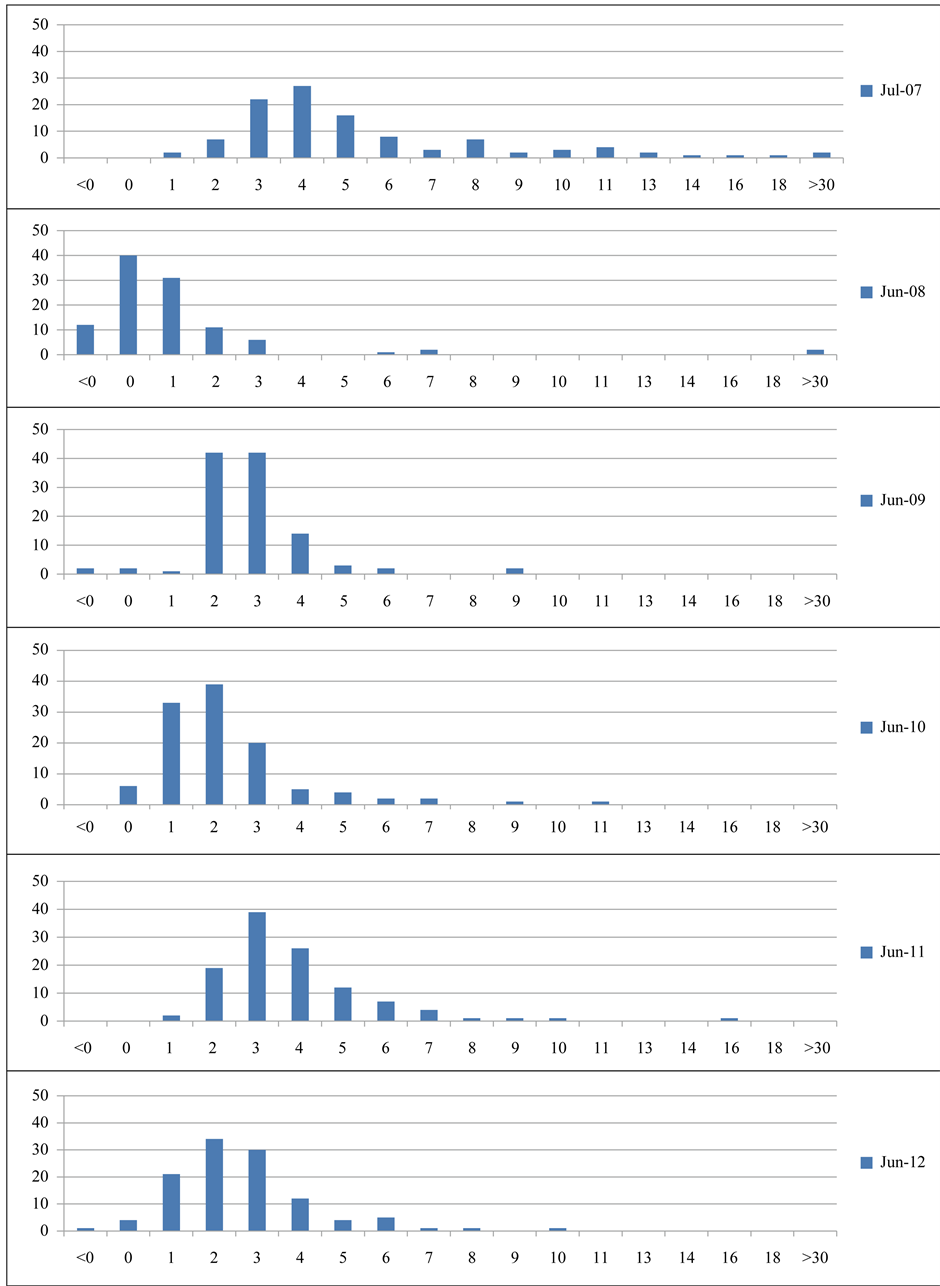
Figure 1. Default distance distribution from 2007 to 2011.
In order to examine the changes of the default distance clearly, we also calculate the average default distance of the real estate companies from 2007 to 2012. From Figure 2, we can see that the average default distance dropped sharply from 2007 to 2008, and it drops from the peak of 8 units to the bottom of −0.53 units. From Oct. 2008, the default distance started to rebound, and it lasted around one year. From 2010 to 2012, the default distance is stable, and it fluctuated within 2 to 5 units. This rising of default distance contributed to the economic stimulation plan. In Nov. 2008, Chinese government announced an economic stimulation plan to overcome the impact of the financial crisis.
5.3. Defaut Distance by Company’s Asset Size
In this section, we will study the difference of default distance between the companies with small asset size and large asset size. Usually, the small size companies are more variable than the large size companies. For example, small companies usually have larger variance of the stock prices. In the research of Chen (Chen, Wang, & Wu, 2010), they found that the small companies have lower default distance than large companies, which means the small company faces a higher default risk than the large company. However, for the real asset company, we found that the result was different with their research.
In order to select the small and large companies, we sort the sample companies by their asset size. And then, we select the top 20 companies in asset size as the large companies and the last 20 companies in asset size as the small companies. We calculate the average default distance of the two groups in time series. From Figure 3, we can see that the default distance of small company is always higher than the large size company from 2007 to 2012, which means that the large company face a higher default risk than the small company.
We find that the asset liability ratio plays an important role here. After examining the asset liability ratio between the large and small companies, we found that the large company usually has a higher asset liablity ratio in the real estate industry (Figure 4), which means a higher risk in the financial view. This high ratio makes the large company’s default distance more than the small size company.
5.4. Default Correlations between Companies
To examine the correlation between different companies, we apply time-varying copula method to this problem, which is one of the improved copula methods. As we introduced before, time-varying copula can present the correlation varying along with time, and the critical point of the time varying copula method is to find the parameters of a time dynamic equation in copula. Usually, the time dynamic equation is constructed by GARCH model.
In the research of default correlations, we still separate the real estate companies into two groups according to their asset size. Here we select the top 20 companies in assets size as large companies and the last 20 as small
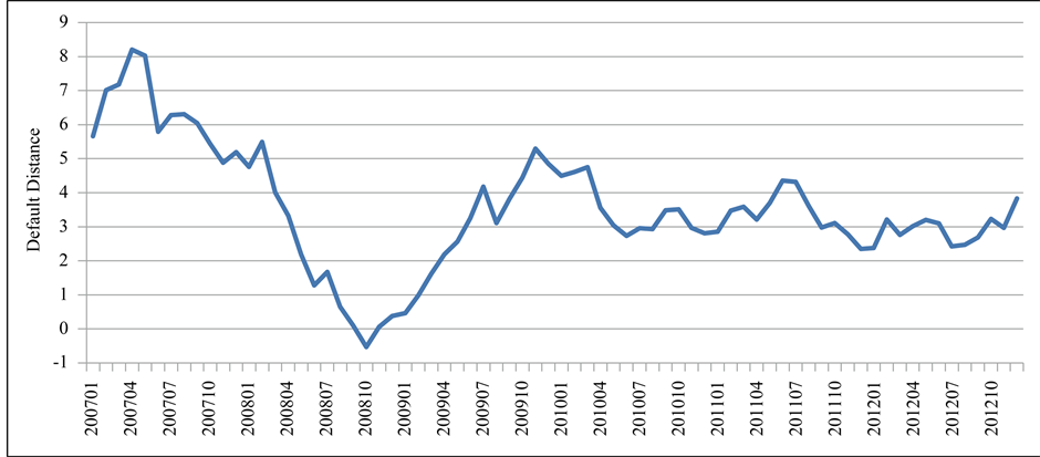
Figure 2. Average default distance from 2007 to 2012.
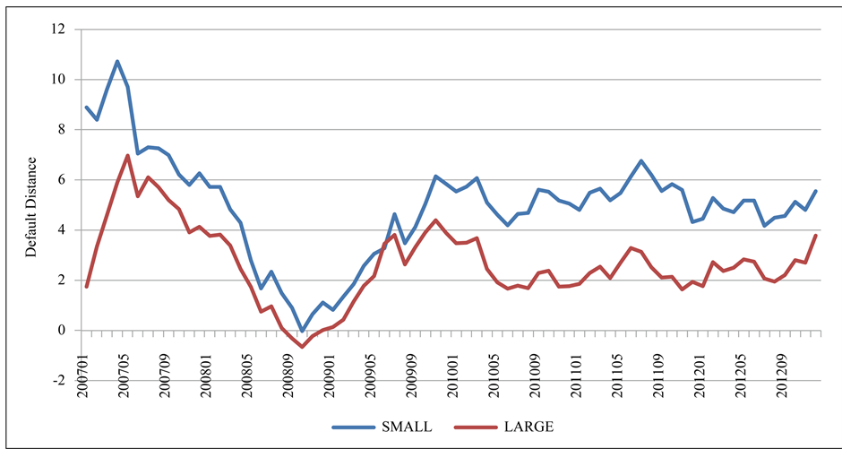
Figure 3. Average defaut distance by asset size from 2007 to 2012.

Figure 4. Asset liability ratio by asset size from 2007 to 2010.
companies. Then, we calculate their average default distance and get the result of time-varying copula.
We estimate the time varying normal copula between large and small asset size companies. Figure 5 shows the normal copula parameter ( ) changing with time. First, we can see that the constant parameter is 0.8 and the time-varying parameter is from 0.75 to 0.9. Both of them show a strong correlation between these two kinds of companies. From the time-varying parameter
 , we can see that during the financial crisis from late 2007 to 2008, the correlation fluctuated around the constant coefficient. Especially, when the financial crisis is severe in 2008, there is a rebound of the correlation.

Figure 5. Time-varying normal copula of large asset size and small asset size companies.
6. Conclusion
In this research, we estimate the default risk fluctuations and correlations of China real estate companies during the finance crisis based on KMV model and time-varying copula. The experimental results show that the default risk not only rises in the finance crisis but also shows some aggregations. Especially, for the real estate companies, the large size companies face higher default risk than the small size companies. This result is contrary to our common understanding, and the asset liability ratio is one of the reasons. These China real estate companies with large size usually have higher asset liability ratio which brings them a higher default risk. At last, we studied the default correlation between companies with different size. The results show that financial crisis did affect the default correlations, while the correlations between the large size and small size companies fluctuated severely during the financial crisis and became smooth after it.
Acknowledgments
This research is supported by National Natural Science Foundation of China (Grant No. 71101083, 71271128 and 71331006); Innovation Program of Shanghai Municipal Education Commission (Grant No. 12ZZ072); Doctor Innovation Funds of Shanghai University of Finance and Economics (Grant No. CXJJ-2012-421); Program for Innovative Research Team of Shanghai University of Finance and Economics.