Keywords:
In this paper, we give a new approach to the finite element approximation for the problem of variational in- equality with noncoercive operator. This problem arises in stochastic control (see [10]). We consider a domain which is the union of two overlapping sub-domains where each sub-domain has its own generated triangulation. To prove the main result of this work, we construct two sequences of subsolutions and we estimate the errors between Schwarz iterates and the subsolutions. The proof stands on a Lipschitz continuous dependency with respect to the source term for variational inequality, while in [5] the proof stands on a Lipschitz continuous dependency with respect to the boundary condition.
The paper is organized as follows. In Sections 2, we introduce the continuous and discrete obstacle problem as well as Schwarz algorithm with two sub-domains and give the geometrical convergence theorem. In Section 3, we establish two sequences of subsolutions and their error estimates and prove a main result concerning the error estimate of solution in the  -norm, taking into account the combination of geometrical convergence and uniform convergence [11,12] of finite element approximation.
2. Schwarz Algorithm for Variational Inequalities with Noncoercive Operator
2.1. Notations and Assumptions
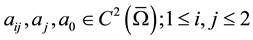
Let’s consider functions
 (1)
(1)
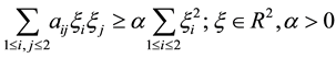
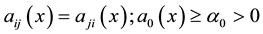
such that
 (2)
(2)
 (3)
(3)
where  is a connected bounded domain in
  with sufficiently regular boundary
 .
.
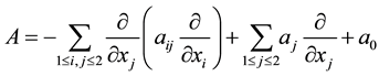
We define a second order differential operator
 (4)
(4)
where the bilinear form associated: 
 (5)
(5)
Let  be a function in
 (6)
(6)
an obstacle
 (7)
(7)
a regular function  defined on
  such that
 (8)
(8)
AM and a nonempty convex set
 (9)
(9)
We assume there exists  large enough and a constant
  such that
 (10)
(10)
Putting
![]() (11)
(11)
then the bilinear form ![]() is strongly coercive.
is strongly coercive.
Let ![]() be the solution of variational inequality (V.I)
be the solution of variational inequality (V.I)
![]() (12)
(12)
which is equivalent to
![]() (13)
(13)
![]() denotes the usual inner product in
denotes the usual inner product in ![]()
We define ![]() the solution of the following V.I
the solution of the following V.I
![]() (14)
(14)
where ![]() and
and ![]() is a mapping from
is a mapping from ![]() into itself.
into itself.
Remark 1. We call quasi-variational inequality (Q.V.I) if the right hand side ![]() depends of solution
depends of solution![]() , in the contrary case we call variational inequality (V.I).
, in the contrary case we call variational inequality (V.I).
2.2. Some Preliminary Results on the V.I Noncoercive
Thanks to [10], the problem (12) has one and only one solution, moreover ![]() satisfies the regularity property
satisfies the regularity property
![]()
We give a monotonicity property of the solution with respect to both the source term, the boundary condition and the obstacle. Let ![]() be a pair of data and
be a pair of data and ![]() the correspond- ing solution of V.I (12).
the correspond- ing solution of V.I (12).
Lemma 1 [10] Under the preceding notations and assumptions (1) to (11), if ![]() and
and![]() , then
, then![]() .
.
Let ![]() be the set of sub-solutions of the Q.V.I, ie all the
be the set of sub-solutions of the Q.V.I, ie all the ![]() such that
such that
![]() (15)
(15)
that is equivalent to
![]()
Lemma 2 [10] Under the preceding notations and assumptions (1) to (11), the solution ![]() of problem (12) is the maximum element of the set
of problem (12) is the maximum element of the set![]() .
.
We show the Lipschitz property, which gives the continuous dependance to the data![]() .
.
Lemma 3 Under the preceding notations and assumptions (1) to (11), we have
![]()
where ![]() is an independent constant of data.
is an independent constant of data.
Proof Firstly, let
![]()
we have
![]()
then
![]()
and
![]()
if we put
![]()
then
![]()
therefore
![]()
Secondly, it is clear that
![]()
and
![]()
![]()
so, due to lemma 1, we get
![]()
which gives
![]()
by changing the roles of ![]() and
and ![]() we obtain
we obtain
![]()
which completes the proof.
Remark 2 If ![]() and
and![]() , then we have
, then we have
![]()
Let ![]() be decomposed into triangles and let
be decomposed into triangles and let ![]() denote the set of those elements;
denote the set of those elements; ![]() is the mesh-size. We assume the triangulation
is the mesh-size. We assume the triangulation ![]() is regular and quasi-uniform. Let
is regular and quasi-uniform. Let ![]() denote the standard piecewise linear finite element space and by
denote the standard piecewise linear finite element space and by ![]() the basis functions of the space
the basis functions of the space![]() . Let
. Let ![]() be the usual restriction operator in
be the usual restriction operator in![]() . The discrete counterpart of (13) consists of finding
. The discrete counterpart of (13) consists of finding ![]() solution of
solution of
![]() (16)
(16)
where
![]() (17)
(17)
![]() is an interpolation operator on
is an interpolation operator on ![]()
We shall assume that the matrix ![]() defined by
defined by
![]() (18)
(18)
is ![]() -matrix [13] (i.e. angles of triangles of
-matrix [13] (i.e. angles of triangles of ![]() are
are![]() ).
).
2.3. The Continuous Schwarz Algorithm
Consider the model obstacle problem: find ![]() such that
such that
![]() (19)
(19)
where ![]() defined in (9) with
defined in (9) with![]() .
.
We decompose ![]() into two overlapping polygonal subdomains
into two overlapping polygonal subdomains ![]() and
and ![]() such that
such that
![]()
and ![]() satisfies the local regularity property
satisfies the local regularity property
![]()
we denote ![]() the boundary of
the boundary of ![]() and
and ![]() The intersection of
The intersection of ![]() and
and ![]()
![]() is assumed to be empty. We will always assume to simplify that
is assumed to be empty. We will always assume to simplify that ![]() are smooth.
are smooth.
For ![]() we define
we define
![]()
We associate with problem (19) the following system: find ![]() solution of
solution of
![]() (20)
(20)
where
![]()
![]()
Starting from ![]() we define the continuous Schwarz sequences
we define the continuous Schwarz sequences ![]() on
on ![]() such that
such that ![]() solves
solves
![]() (21)
(21)
and ![]() on
on ![]() such that
such that ![]() solves
solves
![]() (22)
(22)
where
![]()
![]()
The following geometrical convergence is due to ([2], pages 51-63)
Theorem 1 The sequences ![]() and
and ![]() of the Schwarz algorithm converge geometrically to the solution of the problem (20). More precisely, there exist two constants
of the Schwarz algorithm converge geometrically to the solution of the problem (20). More precisely, there exist two constants ![]() such that for all
such that for all ![]()
![]()
![]()
2.4. The Discretization
For![]() ; let
; let ![]() be a standard regular and quasi-uniform finite element triangulation in
be a standard regular and quasi-uniform finite element triangulation in![]() ,
, ![]() being the mesh size. We assume that the two triangulations are mutually independent on
being the mesh size. We assume that the two triangulations are mutually independent on ![]() where a triangle belonging to one triangulation does not necessarily belong to the other. Let
where a triangle belonging to one triangulation does not necessarily belong to the other. Let ![]() be the space of continuous piecewise linear functions on
be the space of continuous piecewise linear functions on ![]() which vanish on
which vanish on ![]() For
For ![]() we define
we define
![]()
where ![]() denotes a suitable interpolation operator on
denotes a suitable interpolation operator on ![]() We give the discrete counterparts of Schwarz algorithm defined in (21) and (22) as follows.
We give the discrete counterparts of Schwarz algorithm defined in (21) and (22) as follows.
Starting from ![]() we define the discrete Schwarz sequence
we define the discrete Schwarz sequence ![]() on
on ![]() such that
such that ![]() solves
solves
![]() (23)
(23)
and on ![]() the sequence
the sequence ![]() solves
solves
![]() (24)
(24)
We will also always assume that the respective matrices resulting from problems (23) and (24) are ![]() - matrices.
- matrices.
3. Error Analysis
This section is devoted to the proof of the main result of this work. For that, we begin by introducing two auxi- liary sequences.
3.1. Auxiliary Schwarz Sequences
To simplify the notation, we take
![]()
Let ![]() be the solution of discrete V.I
be the solution of discrete V.I
![]() (25)
(25)
where ![]()
![]() is the solution of continuous V.I (21) (resp. (22)) and let
is the solution of continuous V.I (21) (resp. (22)) and let
![]() be the solution of continuous V.I
be the solution of continuous V.I
![]() (26)
(26)
where ![]()
![]() is the solution of discrete V.I. (23) (resp. (24)).
is the solution of discrete V.I. (23) (resp. (24)).
It is clear that ![]() is the finite element approximation of
is the finite element approximation of ![]() Then, as
Then, as ![]() (independent of
(independent of![]() ), therefore, we apply the error estimate for variational inequality (see [11,12]), we get
), therefore, we apply the error estimate for variational inequality (see [11,12]), we get
![]() (27)
(27)
similarly, we have
![]() (28)
(28)
3.2. Sequences of Sub-Solutions
The following theorems will play a important role in proving the main result of this paper.
3.2.1. Part One―Discrete Sub-Solution
We construct a discrete function ![]() near
near ![]() such that:
such that: ![]()
Theorem 2 Let ![]() be the solution of (25). Then there exists a function
be the solution of (25). Then there exists a function ![]() and a constant
and a constant ![]() independent of
independent of ![]() and
and ![]() such that
such that
![]()
Proof Let us give the proof for![]() . The one for
. The one for ![]() is similar. Indeed,
is similar. Indeed, ![]() being the solution of V.I (25) for
being the solution of V.I (25) for![]() , it is easy to show that
, it is easy to show that ![]() is also a subsolution, i.e
is also a subsolution, i.e
![]()
then
![]()
so, due to lemma 2 (discrete case), it follows that
![]() (29)
(29)
where
![]()
setting ![]() and using both remak2 (discrete case) and estimate (27), we get
and using both remak2 (discrete case) and estimate (27), we get
![]() (30)
(30)
which combined with (29) yields
![]()
Thus, we choose
![]()
then
![]()
and
![]()
3.2.2. Part Two―Continuous Sub-Solution
We construct a continuous function ![]() near
near ![]() such that:
such that: ![]()
Theorem 3 Let ![]() be the solution of (26). Then there exists a function
be the solution of (26). Then there exists a function ![]() and a constant
and a constant ![]() independent of
independent of ![]() and
and ![]() such that
such that
![]()
Proof Let us give the proof for![]() . The one for
. The one for ![]() is similar. indeed,
is similar. indeed, ![]() being the solution of V.I (26) for
being the solution of V.I (26) for![]() , it is also a subsolution, i.e.
, it is also a subsolution, i.e.
![]()
then
![]()
so, making use of lemma 2, we obtain
![]() (31)
(31)
where
![]()
Setting ![]() and using both Remark 2 and estimate (28), we get
and using both Remark 2 and estimate (28), we get
![]() (32)
(32)
so, combining (31) with estimate (32) yields
![]()
Finally, choosing
![]()
we get immediately the results.
3.3. L∞-Error Estimate
Theorem 4 ![]() Let
Let ![]() (resp.
(resp.![]() ) be the solution of (21), (22) (resp. (23), (24)). Then there exists a constant
) be the solution of (21), (22) (resp. (23), (24)). Then there exists a constant ![]() independent of
independent of ![]() and
and ![]() such that
such that
![]()
Proof Thanks to theorem 2 and theorem 3, we have
![]()
![]()
therefore
![]() (33)
(33)
moreover
![]()
let ![]() then making use of Theorem 1 and estimate (33), we get
then making use of Theorem 1 and estimate (33), we get
![]()
we choose ![]() such that
such that
![]()
then
![]()
and by inverse inequality, we get
![]()
4. Conclusion
We have established a convergence order of Schwarz algorithm for two overlapping subdomains with non- matching grids. This approach developed in this paper relies on the geometrical convergence and the error estimate between the continuous and discrete Schwarz iterates. The constant c in error estimate is independent of Schwarz iterate n.
References