Accuracy of Stream Habitat Interpolations Across Spatial Scales ()
1. Introduction
Stream habitat data at varying spatial scales provide integral information for lotic management and broad ecologic study. Typically, stream data are collected at multiple spatial scales to provide more complete representation of habitat and allow additional analysis power and ecologic insight [1-3]. The spatial scale at which stream habitat data are collected is important due to connectivity among habitat patches, species occurrence, and life history [3-8]. Because of ecological links between scales, spatial analysis in varying forms has become a staple tool for examining multi-scale stream habitat data [4,9,10]. Collection of stream variables at multiple scales is also necessary for complex analysis of macroinvertebrates, fish habitat relationships, ecological processes, and stream habitat [3,4,7,10,11].
Inability to make inferences at scales other than those collected is linked directly to the unknown amount of accuracy lost when scaling between fine and coarse stream habitat scales [12,13]. Due to the inability of data sets to be scaled for comparative purposes, several data sets are often required for stream habitat spatial analysis at great expense [14]. Data analysis may only be as accurate as the finest scale of data collected [12,15], leading scientists to collect data at the finest scale possible for each study. Unfortunately, an inverse relationship exists between the spatial scale of data and cost to acquire it; the finer the data scale is required, the smaller the area is able to be examined for a given amount of funding.
Utilizing data at various scales has long presented further problems such as pattern analysis and combination of data at varying scales [12,16,17]. Interpolation methods represent a family of spatial statistics able to create map products at multiple scales to aid in ecological pattern analysis and presentation of spatial data [9,18,19]. There are various interpolative methods including inverse distance weighted, several forms of kriging, natural neighbor, point interpolation, trend, and spline to create predictions of stream habitat data [21,22]. Many of these methods have been directly compared on environmental data [23-25]. Comparisons have shown that each method of interpolation has its own strengths in dealing with data of different types and number [19,22,26-30]. Natural neighbor interpolation has shown promise in producing practical maps of streams from small amounts of spatial data [19]. Demonstration of the ability of natural neighbor interpolation to accurately model various scales from a single stream habitat dataset may provide avenues to make multiple scale data collection redundant and opportunity for substantial cost and time savings.
Interpolation creates continuous surfaces from spatial data [20], offering opportunity to alleviate the problem of data gaps in spatial environmental data (e.g. trying to use data across scales). Interpolation provides predictive values of variables in regions which have no data by using information from adjacent regions. This ability provides better potential to use datasets at different scales than those they were initially collected.
Specifically, when selecting stream habitat data variables of depth, flow velocity, and benthic substrate at known locations, natural neighbor interpolation has shown to be accurate [19]. Natural neighbor works well with large datasets and has a nearly identical algorithm as inverse distance weighted interpolation. Natural neighbor interpolation is based on Theissen polygon networks, and weights adjacent data within a specified search radius. It takes a set of spatially located points and creates a grid (raster map) of the area based on the input points at the centroid of each cell. Natural neighbor interpolation works well with stream habitat data such as substrate because depositional patterns in rivers are typically well ordered, and not random [31-33]. Depth, flow velocity, and substrate have a high degree of spatial auto-correlation which further helps prediction accuracy [22,34].
While stream habitat variables of depth, flow velocity, and substrate have been recreated accurately by using natural neighbor interpolation when applied to small amounts of data [19]. There has been no evaluation of the role of spatial scale on stream habitat model accuracy with this type of interpolation. Scaling of stream habitat data typically involves using data across scales in an attempt to understand links between habitat patches, species occurrence, or other environmental variable [11,35- 38]. Such studies often highlight problems caused by aggregating data across ecosystem scales [11,13,16,35,36, 39,40].
This study evaluates accuracy loss of predictive stream models when moving to coarser scales using natural neighbor interpolation. We hypothesize that accuracy retention will be high enough to create practical maps for analysis purposes at scales well removed from the initially collected data scale. A further objective of the study is to examine accuracy of natural neighbor interpolation predictive models at stream sites using data on water depth, water velocity, and benthic substrate at multiple spatial scales. This study will help establish potential for the use of a single dataset across scales in stream habitat modeling. To our knowledge, there has been no such study on scalability of stream habitat data when using natural neighbor interpolation. Our study is relevant to spatial modeling, fish habitat assessment, and stream habitat management because it examines the potential of a single dataset to fulfill analysis needs which would otherwise require multiple datasets at varying spatial scales at an increased cost of time and money. Further, this study emphasizes the rate of accuracy loss between data scales while creating visual maps of stream habitat, which could potentially aid and streamline both data and stream habitat management.
2. Methods
Study Sites and Data Collection
Benthic substrate data were collected from two wadeable streams which were located in the Greater Yellowstone Ecosystem, Gallatin National Forest, Montana, USA. The first of our two sites was located on Little Wapiti creek (111˚16'53.546"W, 45˚2'20.639"N). The Little Wapiti creek site measured nearly 34 meters long by 12 meters wide. The second study site was located on Grayling creek (111˚6'16.407"W, 44˚48'16.878"N). The Grayling creek site measured nearly 29 meters long by 19 meters wide.
Study sites were delineated by grid cells which measured 0.33 by 0.33 meters, or an area of 0.11 m2 resolution per cell, using a fifty meter tape measure, laser rangefinder, and flagging (later removed). For purposes of this study, 0.33 × 0.33 meter grid cells will be referred to by its area, 0.11 m2, or one third (1/3) of a meter squared. This is also referred to as base scale, the finest scale in the study. One third of a meter squared cells were chosen as the base resolution because stream habitat patches could be adequately captured at this scale on a wide variety of stream sizes, including those found in this study. A single piece of rebar was inserted into the bank material on each stream bank and high tensile line was secured to the rebar to guide the tape measure. As each row of data collection was finished the rebar was repositioned upstream to provide support for the next. Starting at the downstream left of each site, values for benthic substrate size, depth, and flow velocity were recorded for each x,y coordinate. Substrate was recorded along a continuous scale in millimeters from 0.05 to >300 mm based on the intermediate axis diameter [41]. Thus, actual values of substrate size were recorded for each 0.11 m2 cell for each study site. Stream depth (cm, top-setting wading rod) and mean water velocity (m/s at 60% depth, MarshMcBirney Flowmate 2000) were measured at the center of each cell. This was repeated until the site was captured in a complete grid of x,y coordinate points (Figure 1, Grayling creek example, upper left inset). All values were recorded in Microsoft Excel. Corner points for each study site were recorded and exported to ArcMap 10. In ArcMap 10, corner points for each study site were georeferenced and exported to Microsoft Excel. Next, x,y coordinates were calculated for the remainder of cells in the site grid and appended to the initial Excel dataset of water depth, flow, and benthic substrate size. Little Wapiti creek had 3630 x,y coordinate points at the base scale, and Grayling creek had 4950 x,y coordinate points at the base scale. The final base scale datasets were imported back to ArcMap 10.
In ArcMap 10, data subsets at 11 additional scales were created from base scale for each study site. Scale increments began at the base scale (0.11 m2) and were increased in size by adding 1/3 of a meter to the length and width of each scale (Figure 2). Thus, base scale of 1/3 of a meter had its cells increased in size to length and width of 2/3 meter by 2/3 meter (0.44 m2) for scale two (Table 1). Scale two in turn had 1/3 of a meter added to its cell width and length to create a one meter by one meter cell scale (1 m2) for scale three (Table 1). This process was continued until 12 scale increments were created, including the final scale of 4.0 m × 4.0 m per cell, or 16 m2 (Table 1). The number of cells used when plotted with scale as the x axis follows a power function with the equation y = 4755.797x−1.923 (Grayling creek), and y = 3438.1x−1.822 (Little Wapiti creek) (Table 1).

Figure 2. Coordinates of centroids of each cell used to created natural neighbor interpolations of study sites.

Table 1. Data information used for interpolations including raster cell size. The number of cells used when plotted with scale as the x axis follows a power function with the equation y = 4755.797x−1.923 (Grayling creek), and y = 3438.1x−1.822 (Little Wapiti creek).
Natural neighbor interpolation was run on each scale to create interpolated maps for comparative analysis to the base scale. Natural neighbor maps served as visual and statistical base for scale accuracy comparisons because they have been shown to predict stream habitat data variables depth, and benthic substrate well [19]. When a continuous grid of data is collected at 1/3 m2 trend curves indicate natural neighbor interpolations are 100% accurate, thus allowing the base scale interpolation to be used as a digital representation of reality for effective comparison [19]. Although successively fewer points were used to create interpolations two through 12 (Table 1), values from the interpolated surface from each site were extracted to the original x,y coordinate points from base scale (3630 for Wapiti and 4950 for Grayling) to allow for exact comparison between base and coarser scales at each site. Extraction was accomplished using the extract values to points tool in ArcMap 10.
Each interpolated dataset from scale two through 12, was then subjected to Ordinary Least Squares (OLS) regression (ArcToolbox, ArcMap 10). Regressions were run with predicted values of depth, flow, and benthic substrate (from interpolated scales 2 - 12) as the dependent variable to explain the expected variable (base scale). In this way, OLS regressions provided comparative r2 values for interpolations and residuals for each individual x,y coordinate (the original 3630 for Little Wapiti creek and 4950 for Grayling creek). Using OLS in this way provides quantitative, directly proportional (percent) comparison between base scale and scales two through 12 in the form of r2. Maps of depth, flow velocity, and benthic substrate residuals were created to display positive and negative prediction trends in the form of standard deviation at each x,y location. Mapping residuals is important because it allows for unique examination of regional accuracy of interpolations. Maps were created showing over and under estimation of each coordinate with standard deviation values classes ranging from −2.5 to 2.5. Residual maps were created by performing OLS regression on extracted natural neighbor interpolated values for all scales compared to base scale.
Root mean square error (RMSE) values were then calculated for interpolations at each scale, plotted, and appropriate trend lines applied to all predicted habitat values (depth, flow, benthic substrate) (Figures 3-7). Plotting of RMSE values for each scale shows decay of accuracy for each scale effectively. Root mean square error compliments r2 values because RMSE decreases as proportional r2 increases. It is important to note that unlike r2 values from interpolations, r2 values on RMSE graphs indicate log trend line fit, and not proportional accuracy of interpolations at each scale. Substrate, which contains silt, sand, gravel, cobble, boulder, and land, had RMSE values calculated for all substrate sizes combined, as well as for each substrate type to allow better understanding of interpolation accuracy (substrate is often discussed in terms of categories, though collected in the form of continuous data).
3. Results
Accuracy of depth, flow, and benthic substrate RMSE values degraded in a logarithmic linear fashion as data scale used to create interpolations became coarser (0.11 m2 to 16 m2) (Figures 3-7). At both sites, depth and flow interpolations retained accuracy more effectively than for benthic substrate (Table 2, Figures 3-7). Grayling creek maintained lower RMSE values than Little Wapiti creek for flow, similar RMSE values for depth, and nearly identical RMSE values at all scales for benthic substrate (Figures 2-6). As scale of data (and number of data points) used to create interpolations became coarser, range between maximum and minimum values for variables decreased. An example of decrease in range of values is shown through depth; by the coarsest scale the range of depths produced by interpolations was 0 - 44.9 cm, rather than 0 - 83 cm, a reduction of nearly half. As indicated by r2 values, interpolation accuracy decreased with use of coarser data, but maintained some integrity even as the amount of data used to create maps decreased nearly 99%, 4950 to 43 for Grayling creek and 3630 to 33 for Little Wapiti creek, from base scale to scale 12 for both sites (Tables 1 and 2).

Table 2. Wapiti Creek base scale (0.11 m2) compared to interpolated values from scales 2, 4, 6, 8, 10, and 12.

Figure 3. Root mean square error values for natural neighbor predicted maps of depth values on Wapiti Creek. Scales 1 - 12 are found on Table 1 and range from 0.11 to 16 square meter cell size.

Figure 4. Root mean square error values for natural neighbor predicted maps of flow velocity values on Wapiti Creek. Scales 1 - 12 are found on Table 1 and range from 0.11 at the base scale to 16 square meter cell size used to crease interpolations at scale 12.

Figure 5. Root mean square error values for predicted maps of all substrate values at Wapiti and Grayling Creeks. Scales 1 - 12 are found on Table 1 and range from 0.11 to 16 square meter cell size.
Interpolated surfaces of Grayling and Wapiti creeks provided visual confirmation of a shrinking range of maximum interpolated values as indicated by RMSE (Figures 3-7), r2 (Table 2), and residual standard deviation (Figures 8 and 9). Interpolation results grew less spatially complex as scale became coarser for all habitat

Figure 6. Little Wapiti creek substrate RMSE values with a logarithmic trend line applied showing r2 values for each. Increase in RMSE as scale moves away from the baseline reference scale shows a progressive tapering effect of accuracy loss as predictive scale moves away from the baseline. Sand substrate size maintained the smallest RMSE change between scales.
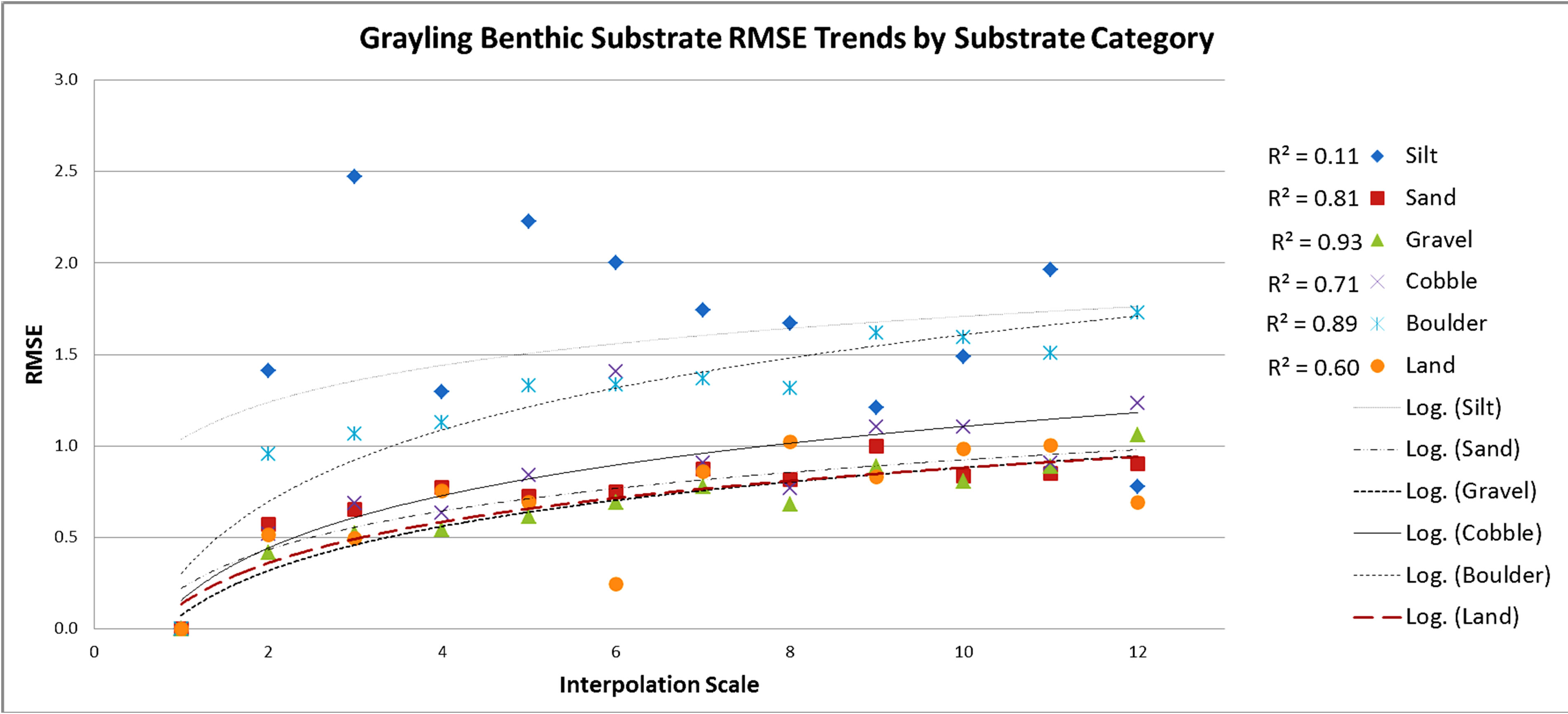
Figure 7. Grayling creek substrate RMSE values with a logarithmic trend line applied showing r2 values for each. Increase in RMSE as scale moves away from the baseline reference scale shows a progressive tapering effect of accuracy loss as predictive scale moves away from the baseline. Sand and gravel maintained the smallest RMSE changes between scales.
variables at both sites. Decrease in spatial complexity was due in part to loss of extreme depths, flow variation and atypically located substrate variables located in the sparser data grid used for coarse scale interpolations (Figure 2). However, location and shape of deep areas, thalweg, zones of like flow, and substrate depositional areas were generally well maintained even to the terminal scale. Maintenance of spatial integrity is indicated by r2 values (percent match) from OLS regressions of each interpolation when compared to base scale (Table 2, Figures 8 and 9).
Ordinary Least Squares regressions demonstrated that all models coarser than base scale tended to underestimate deeper sections of river, and overestimate shallow sections, creating a smoothing effect along both benthic substrate edge boundaries and depth transition zones (Figures 8 and 9). This predictive smoothing effect increased in physical area proportional to the original base scale habitat feature as scale decreased. Another way of illustrating this behavior is that residuals from scale two

Figure 8. Wapiti Creek residual maps showing depth, flow, and substrate standard deviations for each of the 3630 x,y coordinate points at the site. Highly localized regions of standard deviation variation in scale one progress to larger regions of similar standard deviation values as scale becomes smaller, referred to in the text as a smoothing effect. Distribution pattern type of standard deviation types moves from random to clustered.
showed highly localized fluctuation in standard deviation values surrounding habitat zones with high heterogeneity and better lower standard deviation (Figures 8 and 9), while interpolations created from coarser scales saw less regional fluctuation and higher overall standard deviation from the base scale (Figures 8 and 9). Localized variation in standard deviation has decreased because both maximum range of values and the amount of data used for interpolations had both decreased (Table 1). The space between each interpolated data point increased appreciably by the coarsest scale (Figure 2), which also contributed to lack of localized variation. Regressions also demonstrated models created from the coarsest scale, using 99% fewer data points and 145 times more coarse than the original 0.11 m2, were able to match performance of finer scales for some variables (Table 2).
4. Discussion
Our study demonstrated that habitat data collected at a single spatial scale can be successfully used to accurately predict stream habitat at other spatial scales. Our results define the structure of accuracy loss occurring when interpolating coarse resolution with small amounts of fine scale data. As amount of data used to create predictive maps of stream habitat variables departs from the desired resolution, model accuracy decay occurs in a log linear fashion. As accuracy decays, interpolations using less data are able to retain sufficient predictive capability

Figure 9. Grayling Creek residual maps showing depth, flow, and substrate standard deviations for each of the 3630 x,y coordinate points at the site. Abrupt localized changes in standard deviation are more prevalent in scale one. A more gradual change in standard deviation, or smoothing effect, may be seen in scale 12.
required to produce practical (functional, easily interpreted, informative) maps of stream habitat. This is important because adequate accuracy retention between scales affords capability for multi-scale inferences from a single data set. By defining the structure of accuracy loss of natural neighbor interpolations of stream habitat at scales other than the data collection scale through trends in RMSE and OLS regression r2, we have provided a method for estimating the amount of accuracy lost by interpolating across scales.
By observing the combined results of RMSE trends and residual values as a guide to natural neighbor interpolative inaccuracies, it is possible to see a detailed progression of errors caused by departure from initial scale when interpolating stream habitat variables. Identifying a cause for error propagation is valuable because the source of error in environmental predictive models is not always readily apparent. Maps of interpolations and regression residuals also aid in clarifying the scalability of stream habitat variables by showing specific locations of strong and weak model predictions when moving between scales. This helps quantify what detail is eliminated when using data at a coarse scale, an issue important to ecological studies [12,15,36]. The ability to understand accuracy loss when interpolating at coarser scale is better understood, thus increasing the value of a single dataset.
5. Conclusion
This study indicated that the initial scale of collected data and stream size influence the range of scales at which the data set retains usefulness for predictive purposes. For instance Little Wapiti creek showed a drop in predictive accuracy below 60% at the fifth scale removed (from the original) for all habitat variables. The Wapiti site encompassed a series of three pool/riffle zones, while Grayling creek was a single pool riffle interface (three to four times the scale of Little Wapiti). Because of stream size difference in the study, results may have identified presence of a threshold for predictive accuracy purely associated with stream size. This makes ecological sense, in which a larger order stream may have proportionally larger habitat patches which in turn maintains any scale’s predictive accuracy at further reaching scales.
Maintaining spatial integrity of site boundaries and habitat transition zones though interpolations at varying scales from a single dataset was shown to be possible in this study. Spatial integrity is important because it allows accurate measurement of area of available habitat. In streams, the amount and distribution of available habitat are closely tied to species occurrence and species diversity, and their examination aids in ecological study at varying spatial scales [5,6,42-45].
An important question with respect to accuracy of stream habitat models, and perhaps all models, is what level of accuracy is acceptable. This paper does not attempt to answer that question, it only helps quantify the level of accuracy possible and identify details and accuracy lost during the collection and analysis process. Acceptable accuracy is often a function of the question being asked and may vary greatly [44]. Though we do not advocate a particular level for acceptable accuracy in this study, the ability to scale a single habitat data set to a scale far removed from the original and still maintain accuracy, is a valuable tool for stream management and assessment purposes.
6. Acknowledgements
We thank Mike Strager for input on the scientific and editing processes. We thank Richard Sheehan for data collection assistance and Nicole Ten Eyck for recording of data. Reference to trade names does not imply endorsement of commercial products by the US government.