The Finite-Element Modeling of Dynamic Motions of a Constraint Wind Turbine and the System Diagnosis for the Safety Control ()
1. Introduction
To meet high requirement of the structure of modern control systems and to satisfy the reliability of a system, first of all, it is strongly necessary to introduce the mathematical precise description of the given system. Given system used the “Finite Element” which involved the characteristics of the kinetics and kinematics. Especially, when the interest comes to the dynamic behavior by high signal amplitude or various operating points, the safe operation is getting more and more important. This is obviously verified when a part of systems suddenly goes out of function. It can cause an entire system defect, and this is able to bring up a dangerous situation for employee and material losses. To take precautions against these kinds of troubles, many scientists in the world have been making efforts for a long time. For this, it required the inspection during the operation: certainty and system assessment. Only by this way, the sudden appearance of defects and the alteration of the processes can be found out, and the reason for the troubles and the place are detected (Fault Detection and Isolation, FDI). It is important that the fault must be sensed early enough for avoiding the damages in the system (Fault Detection, Isolation and Accommodation, FDIA). When this process goes without man’s help, it’s called automated fault detection, in another word, “gnosis”. Under meaning of fault, we can understand that every abnormal derivation or divergence from the required process behavior and the abrupt fault is meaningful for the safe operation. The FDI process needs certain characteristics being able to give the threshold of the decision: residuum and residue. The method of fault estimated by using the Hardware-redundancy is very costly and less practicable. The model-based methods were presented by [1]. The methods by creating the parameters or state space estimate were given in [2]. There have been some other ways to settle the problem with fault through the consideration of the property of the robustness [3]. A practical solution to this problem was the estimation of the states or its velocities by the use of observers which can estimate a system characteristics of linear or nonlinear states and effects as a mode, so called, “Indirect measurement” [4]. In this work, for this procedure, the mathematical model of the concerned physical system which in the operation time consists of a long shaft and two journal bearings at the ends of the shaft, is derived with the significant remarks such as friction, gravitation, and Coriolis force. With the indirect measurements on two bearings, an observer is designed and is going to be used for the system diagnosis through the comparison within phases.
2. Finite Element Modeling of a Constrained Rotor
In order to control and diagnose complex systems, one would like to obtain quantitative mathematical model of a system by symbolic representation involving an abstract mathematical formulation. Though a mathematical model can be adequate for a certain purpose in mind, it never describes the physical phenomenon exactly. Since the final goal of this work is to develop a diagnosis strategy, the inevitable conclusion is that the modeling problem and the diagnosis problem are not independent. Here, the necessary adequate models for the proposed diagnosis policies are built by “finite element models”. These were comprised of the rotor model, the environment model, and model for the interaction between shaft and bearings. Industrial rotors are usually composed of shafts connected by couplings into a kinematic chain with the journal bearing in the operation situation. The shafts can be either cylindrical or revolute, and are driven by given actuators. In this work only cylindrical shaft will be considered. For the purpose of modeling, the three interacting parts such as the blade of the wind driver, the transmission, and the bearings which are connected with the shaft is considered first as an example of the physical model, the (see Figure 1) shaft is modeled

Figure 1. A constraint rotor system with bearings
into N(=7) segments of shaft i.e. N(=7) sub-finite systems in the numerical matrix form (see Figure 2).
Each one is called a subsystem. At both ends of the shaft, there exist dynamics of the bearings. They have the task of system control. For the initial data needed in the operating system, the displacements of the journals are measured up on the bearings at the left and the right side of the shaft (see Figure 1).
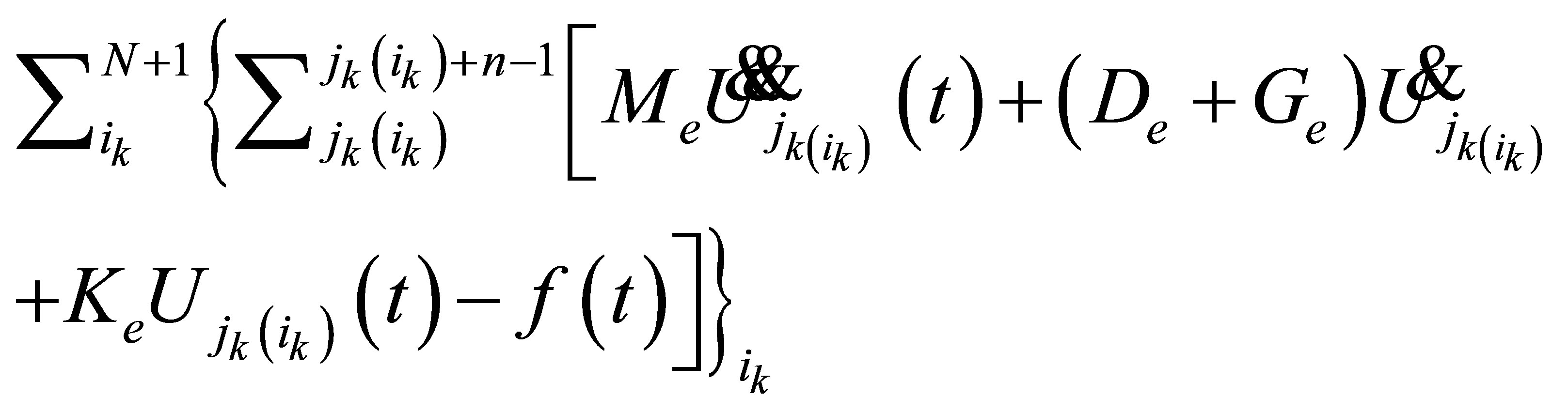
Assuming that the material properties are homogenous, the energy balances, which include the inner kinetics energy, the inner transform energy, damp energy and the energy from outside, are set up for the mathematical description in form of differential equation as following
 (1)
(1)
 (2)
(2)
 (3)
(3)
Here,  and
and  denote the runninr numbers of the finitemente and the initial number of the subsystem
 :mass matrix, and
 :
:
stiffness matrix of undamaged section.
 ,
, : matrix of the damping and gyroscopic matrix
 ,
,  ,
, :
:
displacement vector, velocity vector, and acceleration vector of the system  input vector, and vector of the nonliearities caused by unexpected influence
 :
:

Figure 2. A consistent matrix with bearings.
degree of freedom of considered elementary subsystem. The consistent matrix is built.
From now on, the index will be left out with respect to the whole dynamic system. The dynamic behavior of joint system can be modeled by analogy to [5] as follows
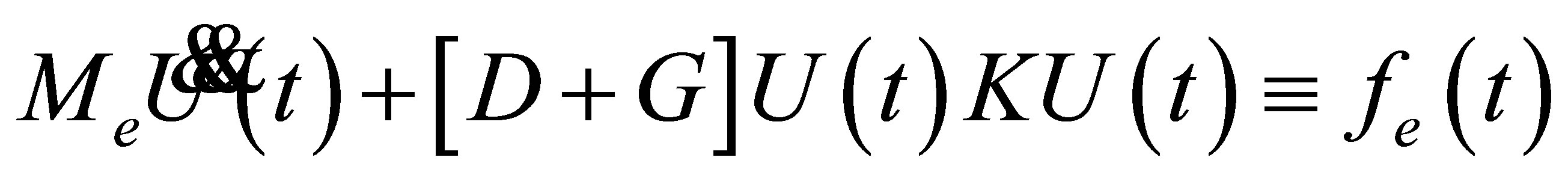 (4)
(4)
The geometrical data and other detailed information are given in the appendix. It is normally convenient for further operation to write the equation above via state space notation  the nonlinearities of the motion created by any defects in system.
 (5)
(5)
The equation of the measurement is given by
 (6)
(6)
 (7)
(7)
where,  is
is  dimensional system matrix which is responsible for the system dynamic with
  and . B is the input matrix in the form as:
 (8)
(8)
The factors  and
and  denote mass unbalances in x and y coordinates respectively as follows
 (9)
(9)
 (10)
(10)
 is the output vector and the measurement matrix C(t)
  presents
  dimensional measurement matrix, respectively. Tie mass as an input is given as follows
 (11)
(11)
 denotes
  dimensional vector of the excitation inputs due to gravitation and unbalances.
Here, the vector  and
and  characterizes the
  dimensional vector of nonlinear functions due to the fault such as mass unbalance and crack, respectively.
  and
and  are the input matrices of the linear and the nonlinearities, and the order of
  is of
is of . It is presupposed that the matrices
  the vector
  and
and  are already known. Now it remains to reconstruct the unknown line arvector
  and nonlinear vector
  which mentions the disturbance force caused by a fault such as mass unbalance and crack. The basic idea is to get the signals from
  approximated by the linear fictitious model, see [6,7]. In terms of the fictitious model, an observer [7] is designed and to get a signal phase an estimator
 (12)
(12)
Is built. For the guarantee of the observer ability of estimator, the requirement:
 (13)
(13)
 (14)
(14)
and the requirement of the control ability
 (15)
(15)
must be satisfied. The output equation for the measurement is presented as follows.
 (16)
(16)
where matrices  and
and  are the gain matrix of the observer. The above Equation (12) means that the observer consists of a simulated model with a correction feedback of the estimation error between real and simulated measurements. The matrix
  has
has . dimensions and represents the dynamic behavior of the elementary observer. The asymptotic stability of the elementary observer can guaranteed by a suitable design of the gain matrices
  and which are possible under the conditions of detect ability or
  observability of the extended system. To enable the successful estimation under the asymptotic stability, the eigenvalue of the considered observer
  must be settled on the left side of the eigenvalue of the given system
  to make the dynamic of the observer faster than the dynamic of the system. The fictitious model of the fault behaviors is able to be designed using integrator model [7,8] based on the chosen crack model as follows. The observer gain matrices
  and
and  can be calculated by pole assignment or by the Riccati equation [4] as follows.
 (17)
(17)
 (18)
(18)
The weighting matrix  and
and  has to be suitably chosen by the trial and errors.
3. Design of the Estimator
In the above section it has been studied how to design the elementary estimator for the detection at a given local position. It means that a certain place on the shaft is initially given as the position. The elementary estimator on the bearing has to survey not only the assigned local position but also any other place on the shaft and to give the signals whether a fault exists or not. As it has been known, it is possible to detect the fault assigned certain place along on the shaft. In the case a fault appears at any subsystem in running time, it must be detected as well. But in many cases, it has been shown that it is impossible or very difficult to estimate the position of the fault at all subsystem on the shaft with one estimator. Generally, it depends on the number of the subsystem and the number of estimator. For the estimation of a position of mass unbalance or crack, an estimator bank based on estimator is designed. The main idea is to reconstruct the related forces of a mass unbalance or crack from certain local position to the arranged elementary estimator. This is main task in this section. The structure of the estimator considered is in the work [7,8] presented. It consists of a few elementary estimator depends on the number of the subsystem is modeled. Every elementary estimator which is distinguished from the distribution vector  gets the same input (excitation)
  and the feedback of the measurements, and is going to be set up at a suitable place on the given system. For the appreciate arrangement of Beo, the distribution matrix on the analogy of (15) has been applied. In this way the estimator bank is established with the estimator. To estimate the local place of the fault, there are two steps. First of all, the estimator must be observable to certain local place in the meaning of the asymptotical stability in the system. The requirement has been satisfied by the criteria from [7,8]. This means that the estimator has to be capable of estimating the fault at any location, where estimator is situated on the given system. The unknown fault position is to be found by the estimator arranged in a certain local place with the related crack forces resulting from the crack. To guarantee this condition (14) is supposed to be fulfilled. In this work three estimators are arranged on the left and right bearings
 (19)
(19)
The unknown position of a fault is found by the estimator according to the related forces, displacement, and torque of some other location on the shaft.
 (20)
(20)
4. Numerical Evaluation through the Simulation on Rotating Shaft
The estimator bank consists of two elementary estimators. The 1st estimator A is situated at the left bearing and 2nd estimator B is placed at the right bearing. The criteria to detect a fault, it is necessary to choose the maximal magnitude of the phase from all estimators by the comparison among the phase turned out: forces, displacements and torque. In the case, the estimator shows none of the force, there is not any mass unbalance in this system considered. If any one of the estimator gives the signal of a force the system has a crack in a corresponding position. The figure illustrates the phases with the mass unbalance under the rpm (107.5). As the 1st example, the nominal system behavior is considered with given mass unbalance is at the 1st of the node in the system.
The y axis shows the force which denotes nonlinearity and the x axis illustrates the corresponding torque. This phase is nominated as a phase of zero fault. The Figure 3 shows that the estimator recognizes the non existence of a fault. By the comparison of the forces, there is some difference between estimated and simulated phase. However, the derivation is small enough and acceptable.
The results in the Figure 4 describe the fault existence (force of mass unbalance) in the 2nd node under the influence of a crack in the runtime operation. Up to 3 [sec], the forces of mass unbalance and crack have been overlapped. This denotes that mass unbalance and crack exist in the same place (node) on the shaft. It has been already mentioned that the breathing direction of a crack and the position of the mass unbalance on the radius of the diameter of shaft are on the same line. By the comparison, the Figure 3 with Figure 4, it is clear to appear a defect. The result in the Figure 5 illustrates the appearance of the fault as phase 4th node: the forces of mass unbalance, in the middle of the shaft.
The result in the Figure 6 tells us the coming up of the fault as phase: the forces of mass unbalance, the forces of mass unbalance, in the 1st node under the influence according to the same direction between mass unbalance and the crack on.
5. Conclusion
From physical model, the mathematical model of the rotating shaft with bearings using the energy balances, which
include the inner kinetics energy, the inner transform energy, damp energy and the energy from outside setup for the mathematical description in forms of differential equation, has been presented. Based on this mathematical model, the elementary observer with the measurement only on the bearings and the observer bank have been developed. With this observer bank, the estimation of the fault has been detected in phase. The above method gives a clear relation between the shaft with a mass unbalance and the damaged shaft by a crack and the phenomena caused in phase by means of the measurement at both bearings. Successful theoretical results have been given in graphics. The forces and torques in the results are the internal one, which have been reconstructed as disturbance forces created by the mass unbalance and crack. It has been theoretically shown that it is possible to estimate localization of a mass unbalance with the opposite direction of a crack. The suggested methods are very significant not only for the further theoretical research and development but also for the transfer in experiments.