1. Introduction
Diffuse Optical Tomography (DOT) provides an approach to probing highly scattering media such as tissue using low-energy near infra-red light (NIR) using the boundary measurements to reconstruct images of the optical parameter map of the media. Low power (1 - 10 milliwatt) NIR laser light, modulated by 100 MHz sinusoidal signal is passed through a tissue, and the existing light intensity and phase are measured on the boundary. The predominant effects are the optical absorption and scattering. The transport of photons through a biological tissue is well established through diffusion equation [1-6] which models the propagation of light through the highly scattering turbid media.
The forward model frequently uses light transport models such as stochastic Monte Carlo simulation [7] or deterministic methods such as radiative transfer equation (RTE) [8]. Under certain conditions such as , the light transport problem can be simplified by the diffusion equation (DE) [9]. The RTE is the most appropriate model for light transport through an inhomogeneous material. The RTE has many advantages which include the possibility of modelling the light transport through an irregular tissue medium. However, it is computationally very expensive. So the DOT systems use the diffusion based approach. Gauss-Newton Method [2]is most frequently used for solving the DOT problem. The methods based on Monte-Carlo are perturbation reconstruction methods [10-12]. The numerical methods used for discretizing the DE are the finite difference method (FDM) [13], and the finite element method (FEM) [2]. Hybrid FEM models with RTE for locations close to the source and DE for others regions have also been considered [14]. The FEM discretization scheme considers that the solution region comprises many small interconnected tiny subregions and gives a piece wise approximation to the governing equation; i.e. the complex partial differential equation is reduced to a set of linear or non-linear simultaneous equations. Thus the reconstruction problem is a nonlinear optimization problem where the objective function defined as the norm of the difference between the model predicted flux and the actual measurement data for a given set of optical parameters is minimized. One method of overcoming the ill-posedness is to incorporate a regularization parameter. Regularization methods replace the original ill-posed problem with a better conditioned but related one in order to diminish the effects of noise in data and produce a regularized solution to the original problem.
A discretized version of diffusion equation is solved using finite element method (FEM) for providing the forward model for photon transport. The solution of the forward problem is used for computing the Jacobian and the simultaneous equation is solved using conjugate gradient search.
In this study, we look at many approaches used for solving the DOT problem. In DOT, the number of unknowns far exceeds the number of measurements. An accurate and reliable reconstruction procedure is essential to make DOT a practically relevant diagnostic tool. The iterative methods are often used for solving this type of both nonlinear and ill-posed problems based on nonlinear optimization in order to minimize a data-model misfit functional. The algorithm comprises a two-step procedure. The first step involves propagation of light to generate the so-called ‘forward data’ or prediction data and an update procedure that uses the difference between the prediction data and measurement data for the incremental parameter distribution. For the parameter update, one often uses a variation of Newton’s method in the hope of producing the parameter update in the right direction leading to the minimization of the error functional. This involves the computation of the Jacobian of the forward light propagation equation in each iteration. The approach is termed as model based iterative image reconstruction (MoBIIR).
The DOT involves an intense computational block that iteratively recovers unknown discretized parameter vectors from partial and noisy boundary measurement data. Being ill-posed, the reconstruction problem often requires regularization to yield meaningful results. To keep the dimension of the unknown parameters vector within reasonable limits and thus ensure the inversion procedure less ill-posed and tractable, the DOT usually attempts to solve only 2-D problems, recovering 2-D cross-sections with which 3-D images could be built-up by stacking multiple 2-D planes. The most formidable difficulty in crossing over a full-blown 3D problem is the disproportionate increase in the parameter vector dimension (a typical tenfold increase) compared to the data dimension where one cannot expect an increase beyond 2 - 3 folds. This makes the reconstruction problem more severely ill-posed to the extent that the iterations are rendered intractably owing to larger null-spaces for the (discretized) system matrices. As the iteration progresses, the mismatch ( , the difference between the computed and measurement value) decreases.
The main drawback of a Newton based MoBIIR algorithm (N-MoBIIR) is the computational complexity of the algorithm. The Jacobian computation in each iteration is the root cause of the high computation time. The Broyden approach is proposed to reduce the computation time by an order of magnitude. In the Broyden-based approach, Jacobian is calculated only once with uniform distribution of optical parameters to start with and then in each iteration. It is updated over the region of interest (ROI) only using a rank-1 update procedure.. The idea behind the Jacobian (J) update is the step gradient of adjoint operator at ROI that localizes the inhomogeneities. The other difficulty with MoBIIR is that it requires regularization to ease the ill-posedness of the problem. However, the selection of a regularization parameter is arbitrary. An alternative route to the above iterative solution is through introducing an artificial dynamics in the system and treating the steady-state response of the artificially evolving dynamical system as a solution. This alternative also avoids an explicit inversion of the linearized operator as in the Gauss-Newton update equation and thus helps to get away with the regularization.
2. Algorithms
2.1. Newton-Based Approach
The light diffusion equation in frequency domain is,
 (1)
(1)
where  is the photon flux,
  is the diffusion coefficient and is given by
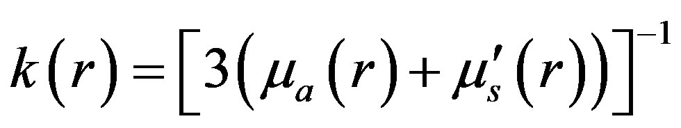 (2)
(2)
 and
and  are absorption coefficient and reduced scattering coefficient
  respectively. The input photon is from a source of constant intensity
  located at
 . The transmitted output optical signal measured by a photomultiplier tube.
The DOT problem is represented by a non-linear operator given by  where
where  gives model predicted data over the domain and M is the computed measurement vector obtained from
  and
and .
.
 (3)
(3)
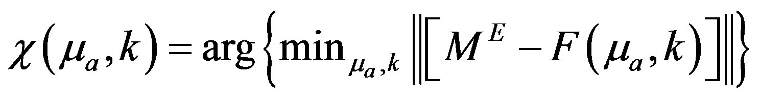
The image reconstruction problem seeks to find a solution  such that the difference between the model predicted
  and the experimental measurement
  is minimum. To minimize the error, the cost functional
  is minimized and the cost functional is defined as [1];
 (4)
(4)
where  is
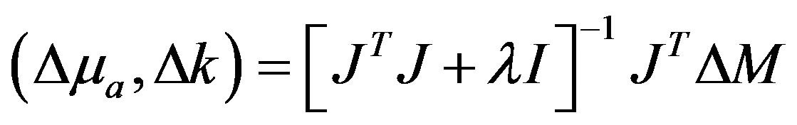
is  norm. Through Gauss-Newton and Levenberg-Marquardt [1,15,16] algorithms, the minimized form of the above equation is given as,
 (5)
(5)
where  is the difference between model predicted data
  and experimental measurement data
 , and J is the Jacobian matrix which has been evaluated at each iteration of MoBIIR algorithm (Figure 1). The above equation is the parameter update expression. In Equation 5, I is the identity matrix whose dimension is equal to the dimension of J
 J.
J.  is regularization parameter and the order of magnitude of
  I should be near to that of J
 J. The impact of noise and
  on the reconstruction is discussed in results section. The Figure 1 gives a flow chart of the approach based on Gauss Newton.
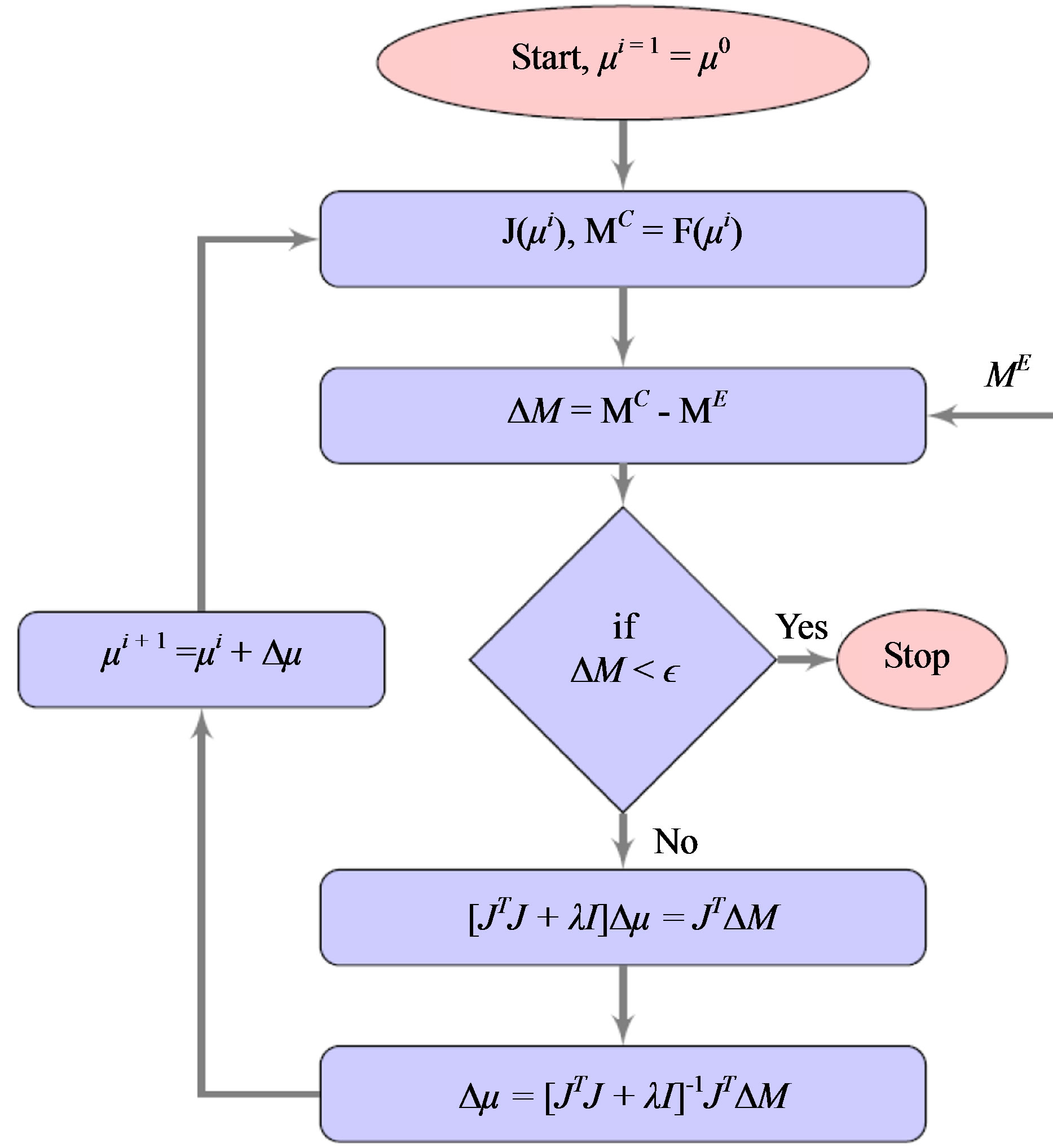
Figure 1. Flowchart for image reconstruction by Newton’s method based MoBIIR algorithm.
2.2. Hessian Based Approach
The iterative reconstruction algorithm recovers an approximation to  from the set of boundary measurements
 . By directly Taylor expanding Equation 3, and using a quadratic term involving Hessian, the perturbation equation can be written as,
 (6)
(6)
where  is the Hessian corresponding to the measurement. For d number of detectors, the above equation can be rewritten as,
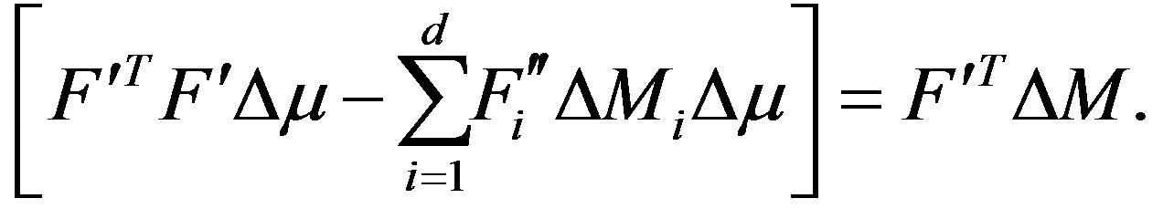 (7)
(7)
The Equation 7 is the update equation obtained from the quadratic perturbation equation. The term  is often observed to be diagonally dominant and can be denoted by
 , neglecting the off diagonal terms. Thus, through the incorporation of the second derivative term, the update equation has a generalized form with a physically consistent regularization term.
2.3. Broyden Approaches
The major constraint of Newton’s method is the computationally expensive Jacobian evaluation [17,18]. The quasi-Newton methods provide an approximate Jacobian [19]. Samir et al [5] has developed an algorithm making use of Broyden’s method [17,18,20] to improve the Jacobian update operation, which happens to be the major computational bottleneck of Newton-based MoBIIR. Broyden’s method approximates the Newton direction by using an approximation of the Jacobian which is updated as iteration progresses. Broyden method uses the current estimate of the Jacobian  and improves it by taking the solution of the secant equation that is a minimal modification to
 . For this purpose one may apply rank-one updates. We have assumed that we have a nonsingular matrix
  and we wish to produce an approximate
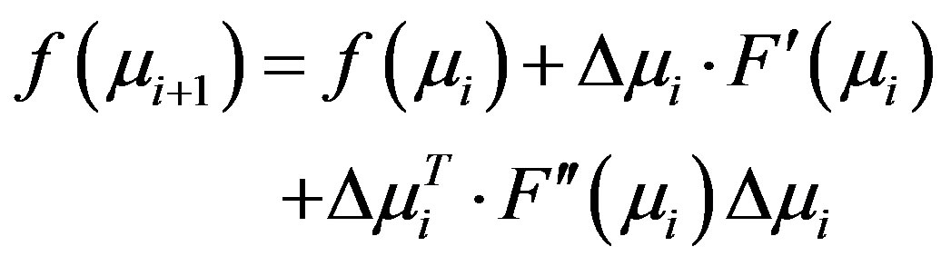
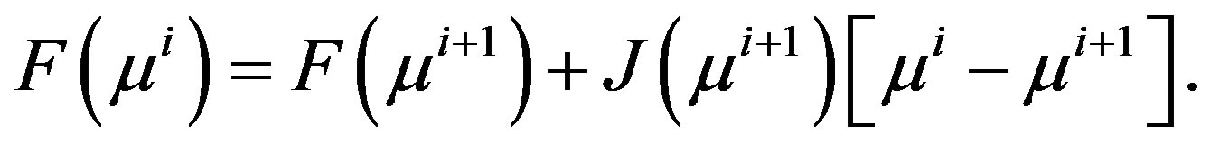
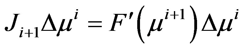
  through rank-1 updates [21]. The forward solution can be expressed in terms of derivatives of the forward solution using Taylor expansion as,
 (8)
(8)
The Broyden’s Jacobian update equation becomes
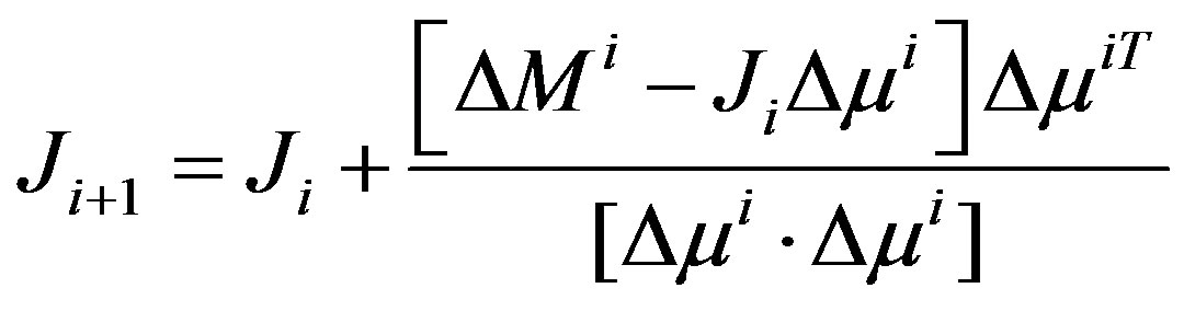
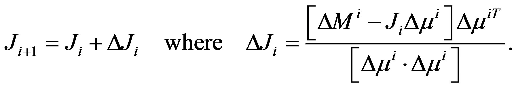 (9)
(9)
Equation 9 is referred to as Broyden’s update equation. In Broyden’s method there is no clue about the initial Jacobian estimate [22]. The initial value of Jacobian  is computed through analytical methods based on adjoint principles. It is found that since Jacobian update is only approximate, the number of iterations required by Broyden method for convergence is higher than that of gauss-Newton methods. This can be improved by re-calculating Jacobian using adjoint method when Jacobian is found to be outside the confidence domain (when MSE of the current estimate is less than MSE of the previous estimate). If the initial guess
  is sufficiently close to the actual optical parameter
  then the
  is sufficiently close to
  and the solution converges q-superlinearly to
 . The most notable feature of Broyden approach is that it avoids direct computation of Jacobian, thereby providing a faster algorithm for DOT reconstruction.
2.4. Adjoint Broyden Based MoBIIR
Least change secant based Adjoint Broyden [23] update method is another approach for updating the system Jacobian approximately.
The direct and adjoint tangent conditions are
 and
and 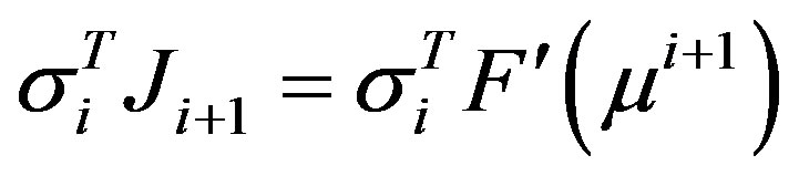
respectively. With respect to the Frobenius norm , the least change update of a matrix
  to a matrix
satisfies the direct secant condition  and the adjoint secant condition
 , for normalized directions
  and
and , and is given as [23]
 (10)
(10)
where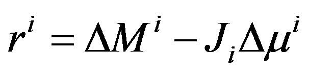 ,
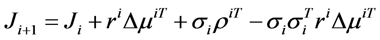
,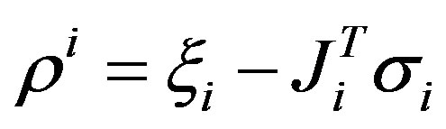 . The rank-1 update for Jacobian update based on adjoint method is given as [5],
 (11)
(11)
The Adjoint Broyden update is categorized based on the choice of . For simplicity, we consider only secant direction [23] which is defined as,
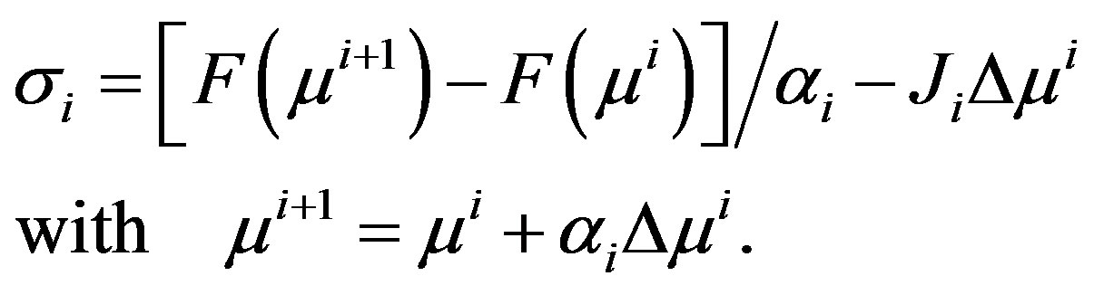 (12)
(12)
where  is the step size and is estimated through line search method. The above equation has been solved in Adjoint Broyden based MoBIIR image reconstruction.
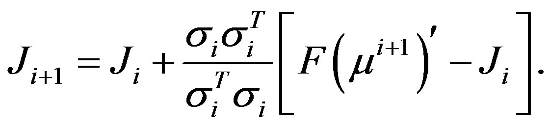
The image reconstruction flowchart using Broyden based MoBIIR is shown in Figure 2. The Jacobian is updated through Equation 9 and Equation 11 for Broyden method and adjoint Broyden method respectively.
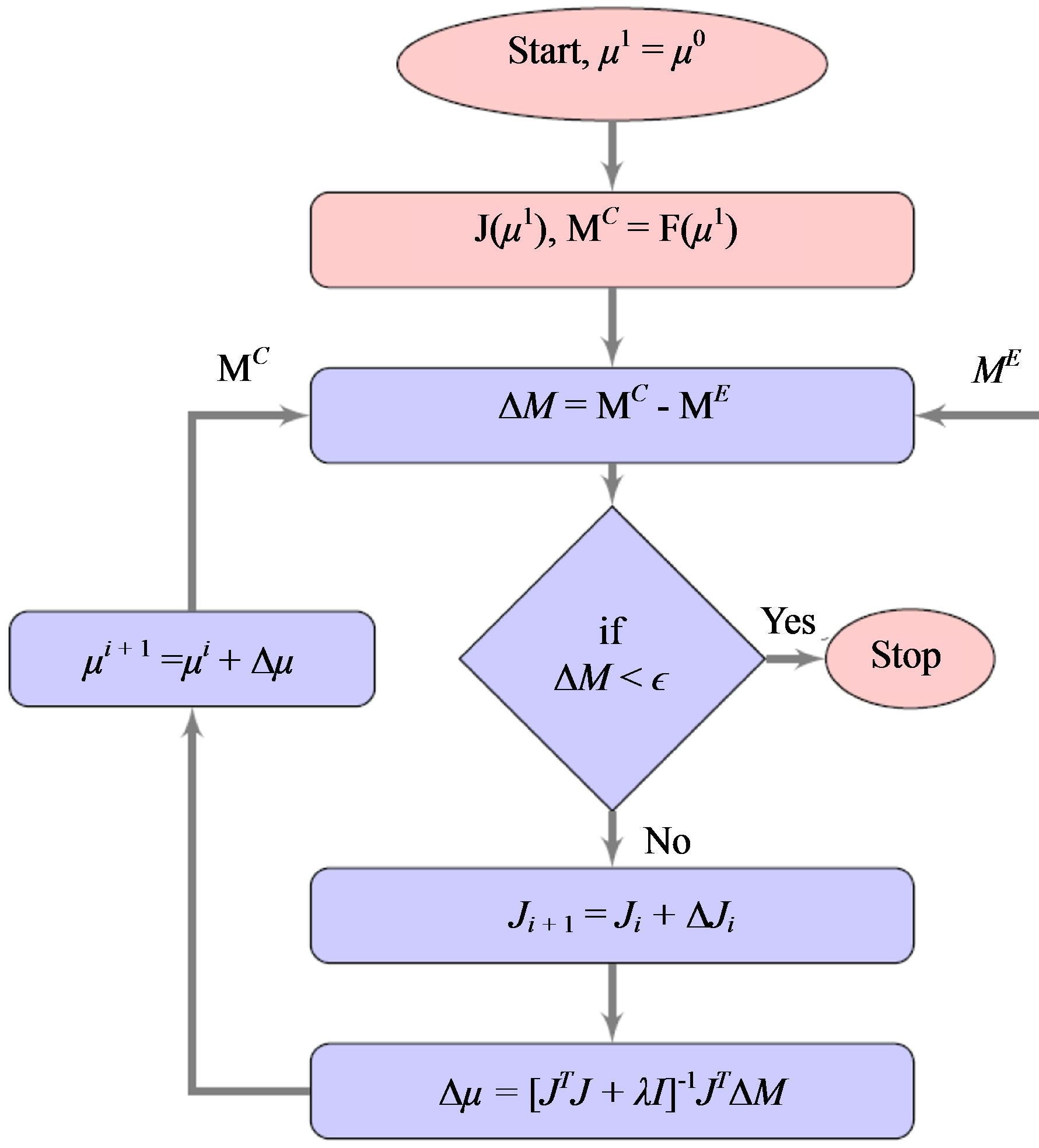
Figure 2. Flowchart for image reconstruction by Broydenbased MoBIIR (Equation 9) algorithm.
2.5. Pseudo-Dynamic Approaches
Diffuse optical tomographic imaging is an ill-posed problem, and a regularization term is used in image reconstruction to overcome this limitation. Several regularization schemes have been proposed in the literature [24]. However, choosing the right regularization parameter is a tedious task. A some what regularizationinsensitive route to computing the parameter updates using the normal equations Equation 5 or Equation 7 is to introduce an artificial time variable [25,26]. Such pseudodynamical systems, typically in the form of ordinary differential equations (ODE-s), may then be integrated and the updated parameter vector recovered once either a pseudo steady-state is reached or a suitable stopping rule is applied to the evolving parameter profile (the latter being necessary if the measured data are few and noisy). Samir et al [5] have used the above approach to arrive at a DOT image reconstruction.
For the DOT problem, the pseudo-time linearized ODE-s for the Gauss-Newton’s normal equation for  is given by:
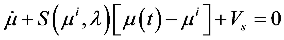 (13)
(13)
where ,
,  ,
,
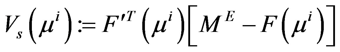 and
and
 when we use Equation 5. For the case where the quadratic perturbation is used (Equation 7), then S is replaced by
 (14)
(14)
We first consider the linear case wherein Equation 5 is used to arrive at the pseudo-dynamic system. While initiating the pseudo-time recursion for , the initial parameter vector
  may be taken corresponding to the background value which is assumed to be known. Equation 13 may be integrated in closed-form leading to the following pseudo-time evolution,
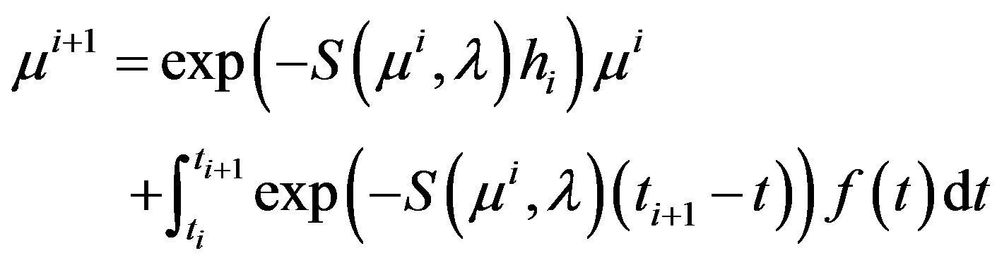 (15)
(15)
where 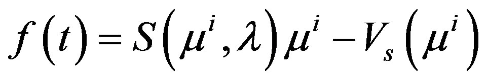 and
and . In the ideal case, when the measured data is noise-free, the sequence
  has a limit point
 , which yields the desired reconstruction. In a practical scenario where the measured data is noisy, i.e,
  with
with  being a measure of the noise ‘strength’. In this case, a stopping rule may have to be imposed so that the sequence
  is stopped at
  (
(
is the stopping time) with .
.
3. Results
Figure 3 gives the reconstruction results with a single embedded inhomogeneity. Figure 3(a) is the phantom with one inhomogeneity. The reconstructed images using Newton-based MoBIIR, Broyden-based MoBIIR and adjoint Broyden-based MoBIIR are given in (b), (c), and (d) respectively.
Figure 4 gives the performance of the algorithm. It is seen that adjoint Broyden converges faster compared to other algorithms. Figure 4(a) shows that Newton, Broyden and adjoint Broyden methods converge at ,
,  and
and  iterations respectively. The cross section through the center of the inhomogeneities is shown in Figure 4(b).