Opportunistic Error Correction: When Does It Work Best for OFDM Systems? ()
1. Introduction
Wireless communication takes place over multi path fading channels [1-3]. Typically, the signal is transmitted to the receiver via a multiple of paths with different delays and gains, which induces Inter-Symbol Interference (ISI). To mitigate the ISI effect with a relatively simple equalizer in the wireless receiver, Orthogonal Frequency Division Multiplexing (OFDM) has become a fruitful approach to communicating over such channels [2,4,5]. The key idea of OFDM is to divide the whole transmission band into a number of parallel ISI-free sub-channels, which can be easily equalized by a single-tap equalizer via using scalar division [6,7]. The information is transmitted over those sub-channels. Each OFDM sub-channel has its gain expressed as a linear combination of the dispersive channel taps. When the sub-channel has nulls (deep fades), reliable detection of the symbols carried by these faded sub-channels becomes difficult.
With the perfect Channel State Information (CSI) at the transmitter, the maximum data rate of a frequency selective fading channel can be achieved by the waterfilling power allocation algorithm [8]. This optimal strategy allocates the transmitted power to the subchannels based on its channel condition. In general, the transmitter gives more power to the stronger sub-channels, taking advantage of the better channel conditions, and less or even no power to the weaker ones [2]. In other words, the total capacity of a frequency selective channel is increased by sacrificing the weak sub-channels. To achieve a certain data rate over a noisy wireless channel, the water-filling algorithm minimizes the transmitted power. Correspondingly, it gives us an energy-efficient transmitter. However, the water-filling algorithm requires the CSI at the transmitter, which may be unrealistic or too costly to acquire in wireless applications, especially in the rapidness of channel changes. Therefore, we propose a novel coding scheme in this paper to maximize the data rate of OFDM systems without CSI at the transmitter, which is realistic to be applied in practical applications and has the same principle as the water-filling algorithm.
Without CSI at the transmitter, the transmitted power is equally allocated to each sub-channel. To achieve reliable communication, error correction codes are usually employed in OFDM systems [8-10]. Over a finite block length, coding jointly yields a smaller error probability than that can be achieved by coding separately over the subchannels at the same rate [2]. This theory has been applied in practical OFDM systems like WLAN and DVB systems [11-15]. The joint coding scheme utilizes the fact that sub-channels with high-energy can compensate for those with low-energy, but its drawback is that each sub-channel is considered equally important. Consequently, the maximum level of noise floor endured by the joint coding scheme is inversely proportional to the dynamic range1. For this par coding scheme, the requirement of the noise floor is even higher to have all received packets decodable.
In a single-user scenario, the noise mainly comes from the hardware, e.g. the RF front and the Analog-to-Digital Converter (ADC) in the receiver. Given a practical wireless system, the noise floor is almost determined. In that case, the maximum data rate of the wireless channel is dependent on the dynamic range of the channel. The higher dynamic range means a lower data rate. Without CSI at the transmitter, we have two approaches to increasing the data rate over a channel with a high dynamic range.
• One is to reduce the noise floor in the RF front and the ADCs. That leads to the high power consumption in the receiver. For the RF front, its power consumption increases by 3 dB if the noise floor decreases by 3 dB [16]. The power consumption in ADCs increases by 6 dB if the quantization noise floor reduces by 3 dB [17]. So, this is not a desirable solution to a battery-powered wireless receiver.
• The other one is to reduce the dynamic range of the channel by discarding a part of the channel in deep fading. Instead of decoding all the information from all the sub-channels, we only recover the data via the strong sub-channels. Just like the water-filling principle, we increase the data rate over the stronger subchannels by sacrificing the weaker ones. In such a case, the total data rate over a frequency selective fading channel can be increased. Correspondingly, the noise floor can be increased to achieve a certain data rate compared to the traditional coding scheme. That leads to an energy-efficient receiver.
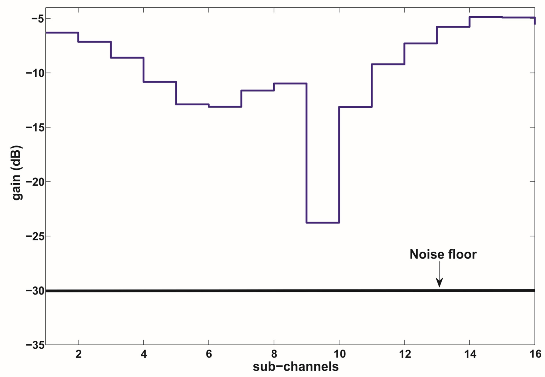
Without CSI at the transmitter, the joint coding scheme does not allow us to give up any part of the channel as it treats each sub-channel equally important. Therefore, we transmit each packet over a single sub-channel. We take Figure 1 as an example to show the advantage of discarding the weak sub-channels. The whole channel is divided into 16 sub-channels and has a dynamic range of around 19 dB. We assume that a packet is encoded by an error correction code with a rate of 
 (a)
(a) (b)
(b)
Figure 1. An example to show the advantage of discarding the weak sub-channels. In this example, each packet is transmitted over a single sub-channel. By discarding the weakest sub-channel, the dynamic range of the channel is reduced by around 11dB. (a) No sub-channel is discarded. (b) 1 sub-channel is discarded.
and it can be decoded successfully when its Signal-toNoise Ratio (SNR) is equal toor larger than . We assume that the maximum noise floor is
  if we want all the packets to be decoded. In such a case, the total data rate
  is equal to
 .However, from this figure, we can see that the weakest sub-channel costs a large part of the dynamic range. By discarding this sub-channel, the dynamic range of the channel is reduced to around 8dB. To compensate for this discarded sub-channel, we use a relatively higher code rate
  to encode each packet that can be decoded if
  With this scheme, the total data rate
  is equal to
 . In this example, if
 , the total data rate
  is increased. Given the same noise floor,
  if
if  the reduced dynamic range (i.e. 11 dB in this example). Otherwise, there is no gain from discarding the weak sub-channels. Obviously,
  is larger than
  in this example. Given the same data rate (i.e.
 ), discarding this sub-channel allows us to increase the noise floor in this example. Equivalently, the power consumption in the receiver is decreased.
Without CSI at the transmitter, the consequence of discarding the weak sub-channels is the loss of packets that are transmitted over those sub-channels. Two solutions can help us to compensate for it. One is to retransmit the lost packets. If the channel changes fast, this approach becomes not efficient and may cost more than that we gain from sacrificing the weak sub-channels. Also, the feedback channel is required, which is expensive in the wireless system. The other approach is to use erasure codes. In such a case, we treat the lost packets as erasures. With the assistance of a certain erasure code, we can achieve reliable communication with an energy-efficient receiver by discarding part of the channel in deep fading. Hence, we propose an energy-efficient error correction scheme based on erasure codes. To apply it to the OFDM-based wireless system, we divide a block of source bits into a set of packets. By treating each packet as a unit, they are encoded by an erasure code. Each erasure-encoded packet is protected by an error correction code that makes the noisy wireless channel behave like an erasure channel. Afterwards, each packet is transmitted over a sub-channel. Thus, multiple packets are transmitted simultaneously, using frequent division multiplexing. With the CSI at the receiver, the receiver discards the packets that are transmitted over the subchannels in deep fading and only decodes the packets with high energy. Erasure codes assist us to reconstruct the original file by only using the survived packets. Therefore, this scheme is called opportunistic error correction.
As mentioned earlier, the joint coding scheme works better than the separate coding over frequency selective fading channels, but it is not straightforward clear whether the opportunistic error correction can endure the higher level of noise floor than the joint coding. In [18], we have compared both in the simulation, whose results have shown that opportunistic error correction has a better performance than the joint coding over frequency selective fading channels. With the same code rate, it has a SNR2 gain of around 8.5 dB over Channel Model A [19] compared to the Forward Error Correction (FEC) layer based on the joint coding scheme in current WLAN standards. However, this new method might not perform better than the joint coding scheme over a narrow-band channel (i.e. a flat-fading channel), as all sub-channels suffer the same fading. There is no gain from discarding some sub-channels. To compensate for the redundancy introduced by erasure codes (i.e. the percentage of discarded sub-channels), opportunistic error correction has to employ a relatively higher code rate to encode each erasure-encoded packet with respect to the joint coding scheme. Given the same type of error correction codes, the one with higher code rate always needs higher SNR to decode correctly. If opportunistic error correction utilizes the same type of error correction codes as the joint coding scheme, it will not perform better than the joint coding scheme over the flat-fading channel. This may be applied to the wireless channel with a low dynamic range. Therefore, it is of great interest to investigate the dynamic range of the channel. This new cross coding scheme shows its advantage over the joint coding scheme. This will tell us what kind of communication environment needs this novel approach. In this paper, we evaluate the performance of opportunistic error correction in the WLAN systems for different dynamic ranges of wireless channels. Its performance analysis is based on simulation results and practical measurements. That will give a good insight whether this new algorithm is robust to the imperfections of the real world that are neglected in simulations.
The paper is organized as follows. Opportunistic error correction is first depicted. We explain why this new method is suitable for OFDM systems and how it works. In section IV-A, we describe the system model by showing how we apply this novel scheme in OFDM systems. After that, we compare its performance with FEC layers from WLAN systems over aTGn3 channel [20] in the simulation. Besides, we evaluate its performance in the practical system in section V. The paper ends with a discussion of conclusions.
2. Opportunistic Error Correction
OFDM enables a relative easy implementation of wireless receivers over frequency selective fading channels [6], but it does not guarantee reliable communications over such channels. Therefore, error correction codes have to be employed in wireless channels. In OFDM systems, coding is performed in the frequency domain. Whether source bits are encoded jointly or separately over all the sub-channels depends on the transmission mode. There are two modes to transmit an encoded packet [21]:
• Mode I is to transmit a packet over a single subchannel. In this case, the coding is done separately over all the sub-channels.
• Mode II is to transmit a packet over all the subchannels. With this method, the coding is performed jointly over all the sub-channels.
Both transmission modes have advantages and disadvantages. Using Mode I, the receiver can predict whether the received packet is decodable since each sub-channel is modeled as a flat-fading channel. The packets transmitted over the sub-channel with low energy can be discarded without going through the whole receiving chain. Correspondingly, the processing power can be reduced. This is a desirable feature for a battery-powered receiver, which cannot be achieved by using Mode II. But Mode I endures a lower Noise Floor (NF) than Mode II to achieve the same quality of communication. As stated earlier, lower NF means higher power consumption in the wireless receiver which is not favorable by a battery-powered receiver.
To have a receiver with both energy-efficient features (i.e. a low processing power from Mode I and a high noise floor from Mode II), we propose opportunistic error correction which combines the separate coding scheme and the joint coding scheme together. Opportunistic error correction is a cross coding scheme. Via erasure codes, source bits are encoded jointly over all the sub-channels; then, each erasure-encoded packet is encoded individually over a sub-channel by error correction codes. This is different from the traditional coding scheme (i.e. the separate coding scheme or the joint coding scheme).
Opportunistic error correction is specially designed for OFDM systems. It is based on erasure codes. Any erasure codes can be applied in it. In this paper, we use fountain codes [22]. Fountain codes are a kind of rateless erasure codes. In [23], MacKay describes the encoder of a fountain coder as a metaphorical fountain that produces a stream of encoded packets. Anyone who wishes to receive the encoded file holds a bucket under the fountain and collects enough packets to recover the original data. It does not matter which packet is received, only a minimum amount of packets have to be received correctly [24]. In other words, with the help of fountain codes, each transmitted packet becomes independent with respect to each other. This allows us to discard some parts of wireless channel with deep fading by transmitting one fountain-encoded packet over a single sub-channel, leading to a reduction of processing power.
Figure 2 shows how opportunistic error correction works. With a fountain code, the transmitter can generate an in-principle infinite sequence of fountain-encoded packets. In this paper, the transmitter generates  number of fountain-encoded packets. Then, each packet is encoded by an error correction code to make wireless channels behave like an erasure channel. Afterwards, each packet is transmitted over a single sub-channel.
At the receiver side, the channel is first estimated. With the channel knowledge, the receiver makes a decision about which packets are to be decoded. We assume that  fountain-encoded packets can go through the error correction decoding. Packets only survive if they succeed in the error correction decoder. The fountain decoder can reconstruct the original file by col-
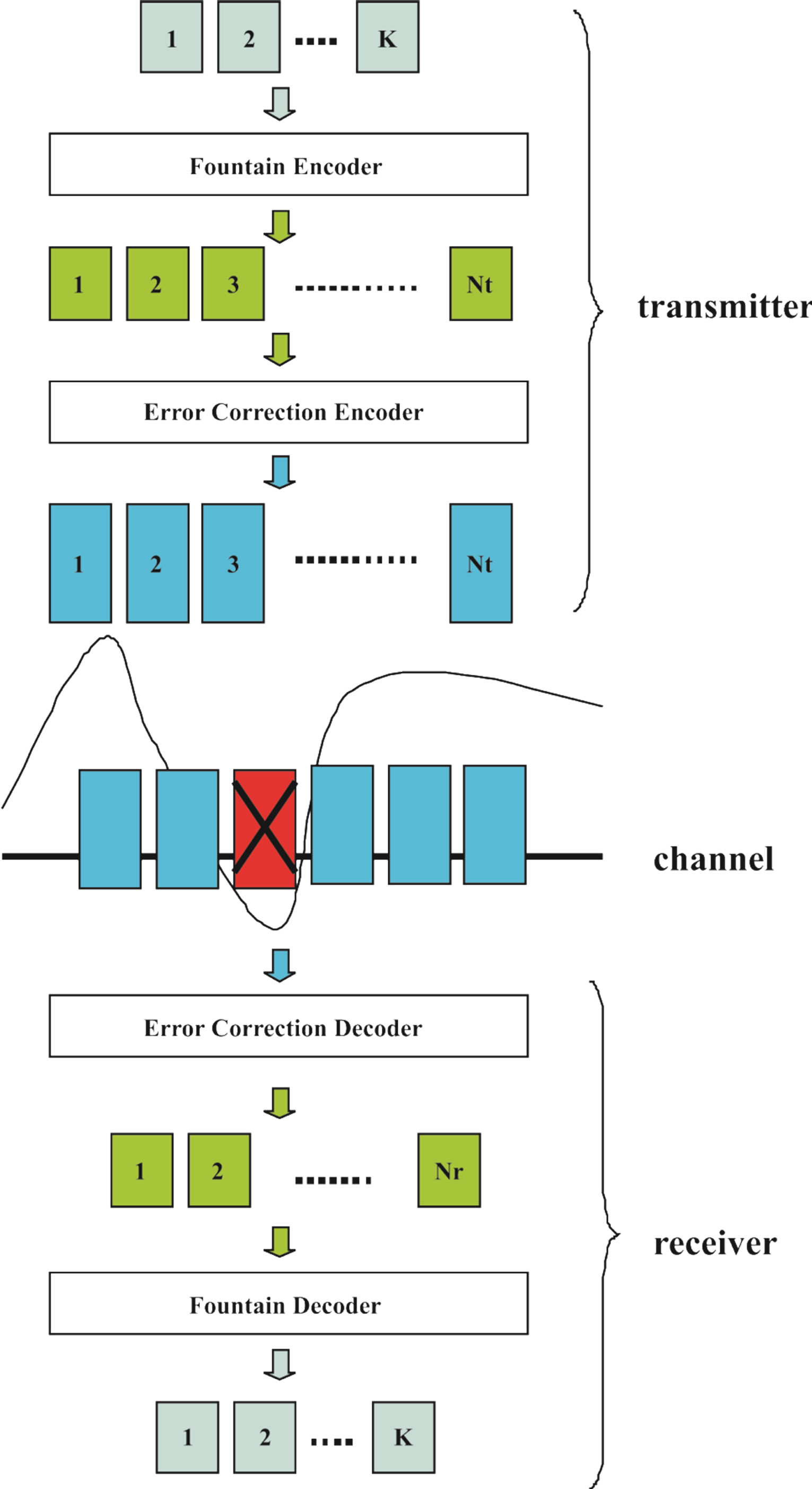
Figure 2. Pictural diagram of opportunistic error correction for OFDM systems.
lecting enough packets. The number of fountain-encoded packets  required at the receiver is slightly larger than the number of source packets
  [23]:
[23]:
 (1)
(1)
where  is the percentage of extra packets and is called the overhead. For high throughput,
  is expected to be as small as possible. However, fountain codes (e.g. Luby-Transform (LT) codes [25]) require a large
  for small block size by only using the message-passing algorithm to decode. For example, the practical overhead of LT codes is 14% when
 , which limits its application in the practical system [26]. In [27], we have shown that the overhead is reduced to 3% by combining the message passing algorithm and Gaussian Elimination to decode LT codes for
 .
.
The performance of opportunistic error correction depends on its parameters (i.e. the rate of erasure codes and error correction codes, the number of discarded subchannels). Given a set of parameters, whether it performs better than the traditional coding scheme depends on the dynamic range of the channel, which will be analyzed in the next section.
3. System Model
Consider a single-user OFDM system with  equally spaced orthogonal sub-channels shown in Figure 3. In the system,
  is the symbol to be transmitted over the
  sub-channel,
  is the
  transmitted symbol in the time domain,
  is the
  channel output,
  is the
  received symbol and
  is the received symbol at the
  sub-channel. As mentioned earlier, the channel noise mainly comes from the hardware in the transmitter and receiver. For simplicity, we assume a perfect transmitter which does not generate any noise to disturb the transmitted signal. However, the discussion below holds more generally.
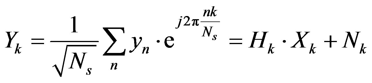
The channel output  can be expressed as:
 (2)
(2)
where  is the number of channel taps,
  is the channel taps and
  is the transmitted symbol.
  is i.i.d uniform-distributed random variables with zero mean and a variance of 1, so
  according to the central limit theorem. The elements in vector
are mutual independent. From the central limit theorem,  can be modeled as a Gaussian-distributed random variable with zero mean and a variance of
 . In this paper, we normalize the channel energy to 1 (i.e.
 ). So,
 .
.
The received symbol is defined by:
 (3)
(3)
where  is the channel noise in the time domain. We assume that
  is an additive white gaussian noise with zero mean and a variance of
 . Due to the additional cyclic prefix in each OFDM symbol, the linear convolution in Equation (2) can be considered as a cyclic convolution [2]. So, after the OFDM demodulation, we can write
  as:
as:
 (4)
(4)
where  is the fading over the
  sub-channel defined by:
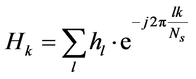 (5)
(5)
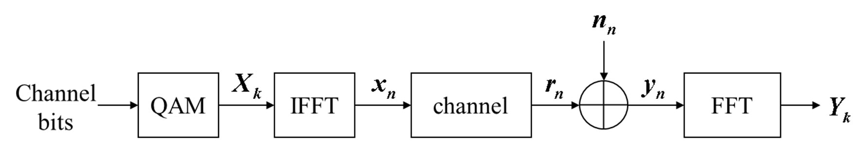
Figure 3. System model showing the transmission over one sub-channel in the OFDM system with ideal synchronization.
 is the noise in the frequency domain and expressed as:
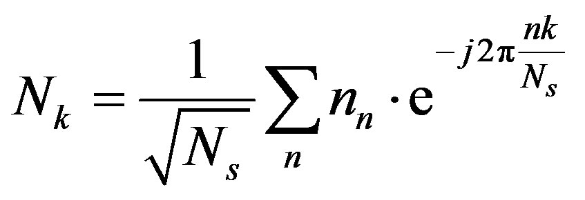 (6)
(6)
According to the central limit theorem,  is a Gaussian distributed random variable with zero mean and a variance of
 . Thus, each sub-channel has the same noise floor, but its SNR is different:
 (7)
(7)
where  is the energy of the
  sub-channel and defined by:
 (8)
(8)
and  is defined by:
 (9)
(9)
Error correcting codes can be applied to mitigate the effect of deep fades. Different coding scheme requires different level of NF (i.e. ) to decode successfully. Assume that
  source packets are encoded by a coding scheme then transmitted over the system as shown in Figure 3. Each packet consists of
  source bits. We encode
  source bits by the following coding schemes, respectively:
• Coding I is to encode them by a Low-Density Parity Check (LDPC) code [8] with a rate of .Each encoded packet is transmitted over a single sub-channel. So,Coding I is a separate coding scheme.
• Coding II is to encode them by the same LDPC code as Coding I. But Coding II is a joint coding scheme as each packet is transmitted over all the sub-channels.
• Coding III is to encode them by opportunistic error correction based on LT codes. We define the rate of LT codes as . Each fountain-encoded packet is protected by a LDPC code with a rate of
  and transmitted over a single sub-channel. To have the same rate as Coding I and II, the number of discarded sub-channels
  can be expressed as:
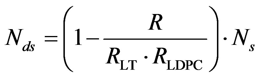 (10)
(10)
where ,
,  and
and .
.
We assume that the LDPC code used in Coding I and II needs  to achieve successful decoding (i.e.
 ) over the AWGN channel. For Coding III, we assume that each fountain-encoded packet can be received correctly if its
 .
.
Because
 ,
, .
.
For the convenience in the analysis, we sort the sub-channels by its energy:

(11)
The dynamic range  of a wireless channel is defined as:
 (12)
(12)
1) Coding I: To have all the packets decodable, the maximum NF for Coding I should be:
 (13)
(13)
2) Coding II: The maximum NF for Coding I is not as straightforward as Coding I. As the joint coding scheme employs the fact that the strong sub-channels can help the weak sub-channels, we use  to classify the weak and strong sub-channels. In such a case,
  means the weak sub-channels and
  means the strong sub-channels. Besides, we assume that Coding II can decode the received packets correctly (i.e.
 ) if the number of weak sub-channels is no more than
 . So, the maximum NF for Coding II is:
 (14)
(14)
As , we have
 . In other words, Coding II (i.e. the joint coding scheme) does not perform worse than Coding I (i.e. the separate coding scheme). If
 , we have
 . In the case of
  (i.e. flat-fading channel or low dynamic range) where
 , we have
 .
.
3) Coding III: With this scheme, each fountain-encoded packet can be received correctly if its SNR is not smaller than . Because
  weak sub-channels can be discarded, the maximum NF for Coding III is expressed as:
 (15)
(15)
The key idea of Coding III is to exchange the code rate of error correction codes with the number of sub-channels to be discarded. If the price paid by using a relatively higher rate of error correction codes can be compensated by the reduced dynamic range, opportunistic error correction (i.e. Coding III) does not perform worse than the traditional coding schemes (i.e. Coding I and II). Equivalently, .if
.if
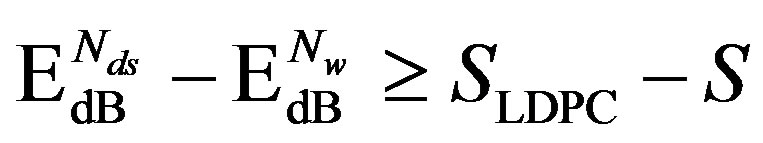 .
.
obviously,  and
and if
if . That might hold for
 . In such a case, there is no reason to apply opportunistic error correction in wireless applications. In the next section, we will search
  in the simulation results.
4. Performance Analysis in Simulation
In this section, we analyze the performance of opportunistic error correction in the simulation. In [18] and [27], we have shown that this new approach works better over Channel Model A [19] than the traditional joint coding scheme from WLAN standards. In this paper, we choose the TGn channel [20] as the channel model. Before checking its overall performance in the TGn channel, let uslook at the statistical characteristics of TGn channels' dynamic range  at different transmission bandwidths (BW). Figure 4 shows the cumulative probability of
  for TGn channels at 5 MHz, 10 MHz and20 MHz. Although they have different BW, their
  mainly distributes in the range of 0 ~ 40 dB (i.e. at a probability of 99%). In this section, we analysis the performance of opportunistic error correction over the TGn channel model at different
  and its overall performance at different BW.
4.1. System Setup
The opportunistic error correction layer is based on fountain codes which have been explained in the above section. This proposed cross layer can be applied in any OFDM-based wireless systems. In this paper, the IEEE 802.11a system is taken as an example of OFDM systems.
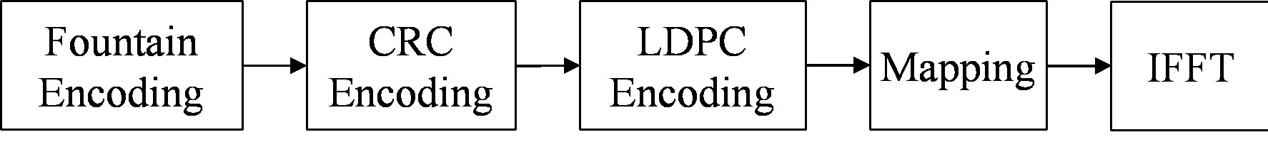
In Figure 5, the proposed new error correction scheme is depicted. The key idea is to generate additional packets by the fountain encoder. First, source packets are encoded by the fountain encoder. Then, a CRC checksum is added to each fountain-encoded packet and the LDPC encoding is applied. On each sub-channel, a fountainencoded packet is transmitted. Thus, multiple packets are transmitted simultaneously, using frequency division multiplexing.
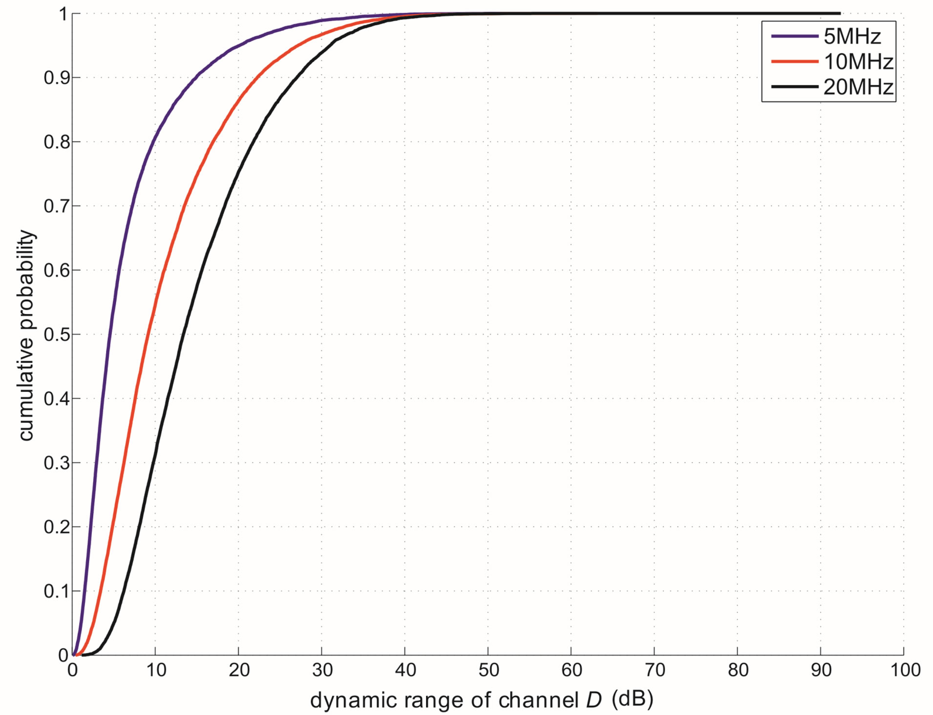
Figure 4. The cumulative distribution curves of the dynamic range  for the TGn channel at 5 MHz, 10 MHz and 20 MHz.
 (a)
(a)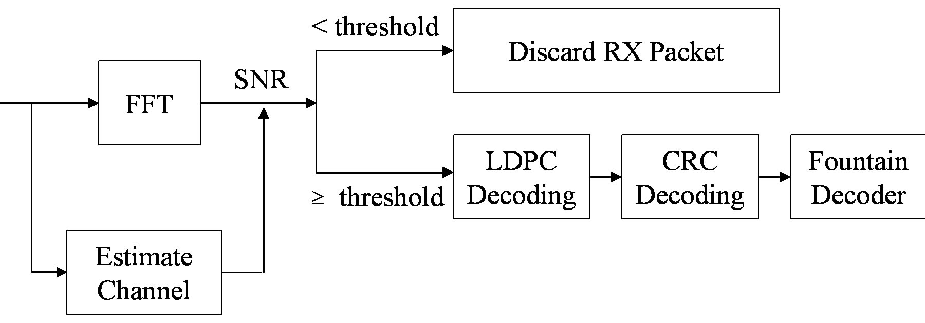 (b)
(b)
Figure 5. Proposed IEEE 802.11a transmitter (top) and receiver (bottom). (a) Transmitter; (b) Receiver.
At the receiver side, we assume that synchronization and channel estimation are perfect in the simulation. If the SNR of the sub-channel is equal to or above the threshold, the received fountain-encoded packet will go through the LDPC decoding, otherwise it will be discarded. This means that the receiver is allowed to discard low-energy sub-channels (i.e. packets) to lower the processing power consumption. After the LDPC decoding, the CRC checksum is used to discard the erroneous packets. As only packets with a high SNR are processed by the receiver, this will not happen often. When the receiver has collected enough fountain-encoded packets, it starts to recover the source data.
4.2. Simulation Results
In this section, we compare three FEC schemes in simulation as follows:
• FEC I: LDPC codes at  with interleaving from the IEEE 802.11n standard [12]
 .
.
• FEC II: fountain codes with the (175,255) LDPC code [28] plus 7-bit CRC using the transmission Mode I, which is the opportunistic error correction layer.
• FEC III: fountain codes with the (175,255) LDPC code plus 7-bit CRC using the transmission Mode II.
Three FEC schemes are simulated as function of the dynamic range  and/or the bandwidth BW by transmitting 1000 bursts of data (i.e. around 100 million bits) over the TGn channel. Each burst consists of 583 source packets with a length of 168 bits. With the same code rate of
 , source packets are encoded by FEC I, II and III, respectively. Afterwards, they are mapped into QAM-16 symbols before the OFDM modulation.
For the case of FEC II and III, each burst is encoded by a LT code (designed by using parameters 
 [23]) and decoded by the message-passing algorithm and Gaussian elimination together. From [27], we know that 3% overhead is required to recover the source data successfully. To each fountain-encoded packet, a 7-bit CRC is added, then the (175,255) LDPC encoder is applied. Under the condition of the same code rate (i.e.
 ), we are allowed to discard 21%4 of the transmitted packets. In FEC II, we transmit one packet per sub-channel. In this case,
  (i.e. 21% of 48 data sub-channels). In FEC III, we transmit each fountain-encoded packet over all the data sub-channels. Similar to FEC II, we are allowed to have a 21% packet loss in FEC III.
4.2.1. Channel at Different Dynamic Range
In total, we compare them under 6 situations: the flatfading channel (i.e. the AWGN channel),  dB,
dB,  dB,
dB,  dB,
dB,  dB and
  dB. Figure 6 shows the simulation results. In the case of the flat-fading channel, we see that FEC I performs better (i.e. a SNR gain of around 2 dB) than FEC II and III as expected. That is because FEC I employs lower code rate of LDPC codes (i.e.
 ) comparing to the LDPC code used in FEC II and III. The same performance has been observed in the case of
  dB, as we can see in Figure 6. Hence, we can say that the joint coding scheme (i.e. FEC I) performs better than the cross coding scheme (i.e. FEC II) at
  dB. Furthermore, there is no difference in the performance between the transmission Mode I and II with fountain codes (i.e. between FEC II and III) at
  dB.
dB.
FEC II starts to show its advantage over the joint coding scheme (i.e. FEC I and III) when  is higher than 10 dB.
• Comparing to FEC I at a BER of  or lower, FEC II has a SNR gain of around 1 dB at
  dB, around 6 dB at
  dB, around 10.5 dB at
  dB and around 13.5 dB at
  dB. From Figure 6, we can see that the performance of FEC I degrades (i.e. a SNR loss of around 6 dB)as
  increases by 10 dB. That does not apply to FEC II.FEC II is more robust to the variation of
 . Only when the dynamic range of the channel
  changes from (10,20]dB to (20,30] dB, FEC II loses around 2 dB in SNR to achieve the error-free quality. From
  dB, there is no performance loss as
  increases.
• Comparing to FEC III at the error-free quality, FEC II has a SNR gain of 1 dB at  dB, 3 dB at
 dB, 7 dB at
  dB and11 dB at
  dB. The performance of FECIII degrades (i.e. a SNR loss of 4 dB) as
  increases by10 dB. That is less than the case of FEC I (i.e. a SNR loss of 6 dB at every 10 dB increase in
 ).
).
Therefore, we can conclude that fountain codes make error correction coding schemes more robust to the variation of .
.
As mentioned before, the key point of opportunistic error correction (i.e. FEC II) is to exchange the code rate of the used error correction codes with the number of discarded sub-channels. Simulation results conclude that there is no benefit to have this tradeoff when the dynamic range of the channel is within 10 dB. The profit starts for
 dB and increases with
 .
.
4.2.2. Channels at Different Bandwidth
In this part, we compare them over the TGn channel with different bandwidth: 5 MHz, 10 MHz and 20 MHz. Figure 4 has presented that different bandwidth has different probability distribution of . The average
  increases with the channel bandwidth. Simulation results are shown in Figure 7, where we can see that FECII works significantly better than the joint coding scheme (i.e. FEC I and III) at any BW. The performance of FEC I, II and III degrades when BW increases. FEC I loses around 3 dB when BW doubles. When BW changes from 5 MHz to 10 MHz, there is a SNR loss of around 2 dB in FEC II and around 4 dB in FEC III. Both FEC II and III lose 1 dB when BW increases from 10 MHz to 20 MHz. In a word, FEC II is less sensitive to the variation of BW than FEC I and III, because the performance of FEC II is more robust to the increase of
 than FEC I and III. Comparing with FEC I at BER of
  or lower, FEC II has a SNR gain of around 11 dB at BW = 5MHz, around 12.5 dB at BW = 10 MHz and around 14.5 dB at BW = 20MHz. The SNR gain increases with BW. With respect to FEC III at the error-free quality, FEC II gains a SNR of 3 dB at BW = 5 MHz, 5 dB at BW = 10 MHz and 20 MHz.
In general, FEC II and III performs better than FEC I at BW = 5 MHz, 10 MHz and 20 MHz. The reason behind is as follows. Due to the variation of the channel, a burst data encounters several channels with different . For the case of FEC II and III, if some part of fountain-encoded packets are lost more than expected ina channel with
 , fountain codes still can recover the original data when the other part of fountain-encoded packets is lost less than expected in the channel with
 . However, this does not apply to FEC I.
5. Practical Evaluation
The C++ simulation results in the above section have shown the performance of opportunistic error correction in comparison with the joint coding scheme (i.e. FEC I and III) over the TG n channel with different  and BW, respectively. C++ simulation, with its highly accurate double-precision numerical environment, is on the one hand a perfect tool for the investigation of the algorithms. On the other hand, many imperfections of the real-world are neglected (e.g. perfect synchronization and channel estimation are assumed in Section IV, which does not happen in the real-world). So, simulation may show a too optimistic receiver performance. In this section, we evaluate its performance in practice to investigate whether opportunistic error correction is more robust to the real-world’s imperfections.
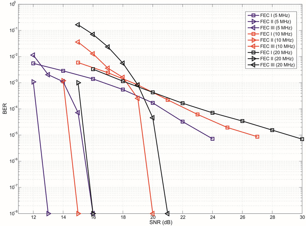
Figure 7. Performance comparison between FEC I, II and III at  over the TGn channel at different bandwidths (i.e. 5 MHz, 10 MHz and 20 MHz). FEC II and III can achieve error-free decoding when the fountain decoder receives enough fountain-encoded packets. We represent BER = 0 by
  in this figure.
5.1. System Setup
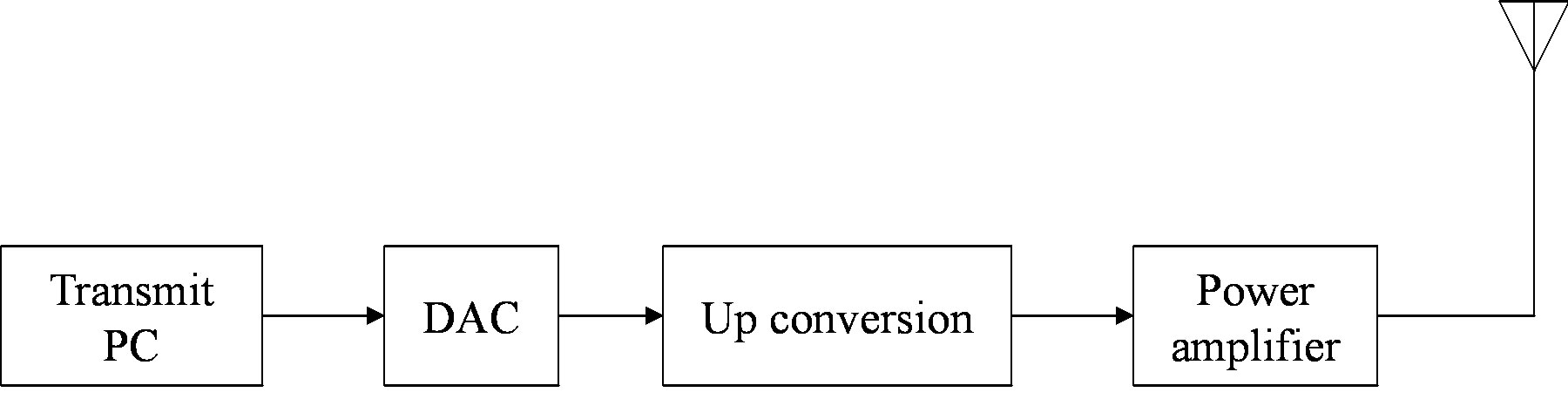
The practical measurements are done in the experimental communication test bed designed and built by Signals and Systems Group [29], University of Twente, as shown in Figure 8. It is assembled as a cascade of the following modules: PC, DAC, RF up-converter, power amplifier, antenna, and the reverse chain for the receiver. In the receiver, there is no power amplifier and band-pass RF filter before the down-converter but a low-pass base band filter before the ADC tore move the aliasing.
5.1.1. The Transmitter
The data is generated offline in C++. The generation consists of the random source bits selection, the FEC encoding and the digital modulation as we depict in Section IV-A. The generated data is stored in a file. A server software in the transmit PC uploads the file to the Ad link PCI-7300Aboard5 which transmits the data to DAC (AD9761)6 via the FPGA board. After the DAC, the base band analog signal is up converted to 2.3 GHz by a Quadrature Modulator (AD8346)7 and transmitted using aconical skirt monopole antenna.
 (a)
(a)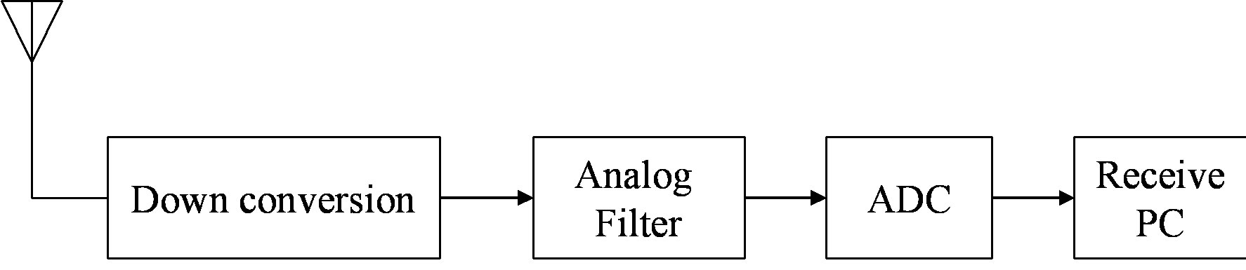 (b)
(b)
Figure 8. Block diagram of the testbed. (a) Transmitter; (b) Receiver.
5.1.2. The Receiver
The reverse process takes place in the receiver. The received RF signal is first down converted by a Quadrature Demodulator (AD8347)8, then filtered by the 8th order low-pass Butterworth analog filter to remove the aliasing. The base band analog signal is quantized by the ADC (AD9238)9 and stored in the receive PC via the Ad link PCI board.
The received data is processed offline in C++. The receiver should synchronize with the transmitter and estimate the channel using the preambles and the pilots, which are defined in [11]. Timing and frequency synchronization is done by the Schmidl & Cox algorithm [30] and the channel is estimated by the zero forcing algorithm. In addition, the residual carrier frequency offset is estimated by the four pilots in each OFDM symbol [31]. After the synchronization and the channel estimation, decoding can start as we describe in Section IV-A.
5.2. Measurement Setup
Measurements are carried out in the corridor of Signals and Systems Group, located at the 9th floor of Building Hogekamp in University of Twente, the Netherlands. The measurement setup is shown in Figure 9. The transmitter (TX) was positioned in front of the elevator (i.e. one of the circle positions in Figure 9), while the receiver antenna (RX) was in the left side of the corridor (i.e. the cross positions in Figure 9). 89 measurements were done inth is scenario with a non-line-of-sight situation. The average transmitting power is around −10 dB m and the distance between the transmitter and the receiver is around 6 ~ 52.5 meters. The measurements were conducted at 2.3 GHz carrier frequency and 20 MHz bandwidth.
In the simulation depicted in section IV, these FEC schemes can be compared by using the same source bits. Different channel bits can go through the same random frequency selective channel. However, itdoes not apply in the real environment. The wireless channel is timevariant even when the transmitter and the receiver are stationary (e.g. the moving of elevator with the closed door can affect the channel). Hence, we should compare them by using the same channel bits.
Because not every stream of random bits is a codeword of a certain coding scheme, it is not possible to derive its corresponding source bits from any sequence of random bits, especially for the case of FEC II and FEC III. Fortunately, the decoding of FEC I is based on the parity check matrix. Any stream of random bits can have its unique sequence of source bits with its corresponding syndrome matrix. The receiver can decode the received data based both on the parity check matrix and the syndrome matrix. So, FEC I can use the same channel bits with FEC II. In such a case, they can be compared under the same channel condition (i.e. channel fading, channel noise and the distortion caused by the hardware.). Therefore, we only compare the joint coding scheme from the IEEE 802.11n standard (i.e. FEC I) with opportunistic error correction (i.e. FEC II) in there al world.
In the measurements, FEC I and II are compared with the same code rate (i.e. ). More than 600 blocks of source packets are transmitted over the air. Each block consists of 97944bits. Source bits are encoded by FEC II. The encoded bits are shared by FEC I as just explained. Afterwards, they are mapped into QPSK symbols10 before the OFDM modulation.
Each measurement corresponds to the fixed position of the transmitter and the receiver. It is possible that some measurements might fail in decoding. Due to the lack of a feedback channel in the testbed, no retransmission can occur. In this paper, we assume that the measurement fails if the received data per measurement has a BER higher than  by using FEC I. For the case of FECII, if the packet loss is more than 21% as expected, we assume that the measurement fails.
5.3. Measurement Results
In total, 89 measurements have been done. There are 7 blocks of data transmitted in each measurement. The estimated  of the channel over those 89 measurements distributes in the range of around 50% of the measurements have
  dB; around 39% of the measurements have
  dB; around 10% of the measurements have
  dB; around 1% of the measurements have
  dB.
dB.
FEC II succeeds in all the measurements but that does not happen to FEC I. Figure 10 shows the percentage of the successful measurements for each . With FEC I, the probability of the successful measurements decreases as
  increases. In the simulation, FEC I works better than FEC II at
  dB, but it does not happen in the real life. FEC I can only achieve a BER of
  or lower in around 93% of the measurements while FEC II gives us the error-free quality in all the measurements at
  dB. That shows FEC II is more robust to the imperfections of the real world than FEC I. Furthermore, FEC I fails in more than 40% of the measurements at
 dB and it cannot survive in the measurements at
  dB. From this point, weal ready can conclude that FEC II works better than FEC I in practice.
Both FEC I and II succeed in 77 measurements, where the SNR of the received signal ranges from 12 dB to 25 dB. In order to investigate whether FEC II can endure higher level of noise floor (i.e. lower SNR) than FEC I, we add extra white noise to the received signal in the software. It is difficult to have the same SNR range in all measurements, so we evaluate their practical performance by analyzing the statistical characteristics of meas-
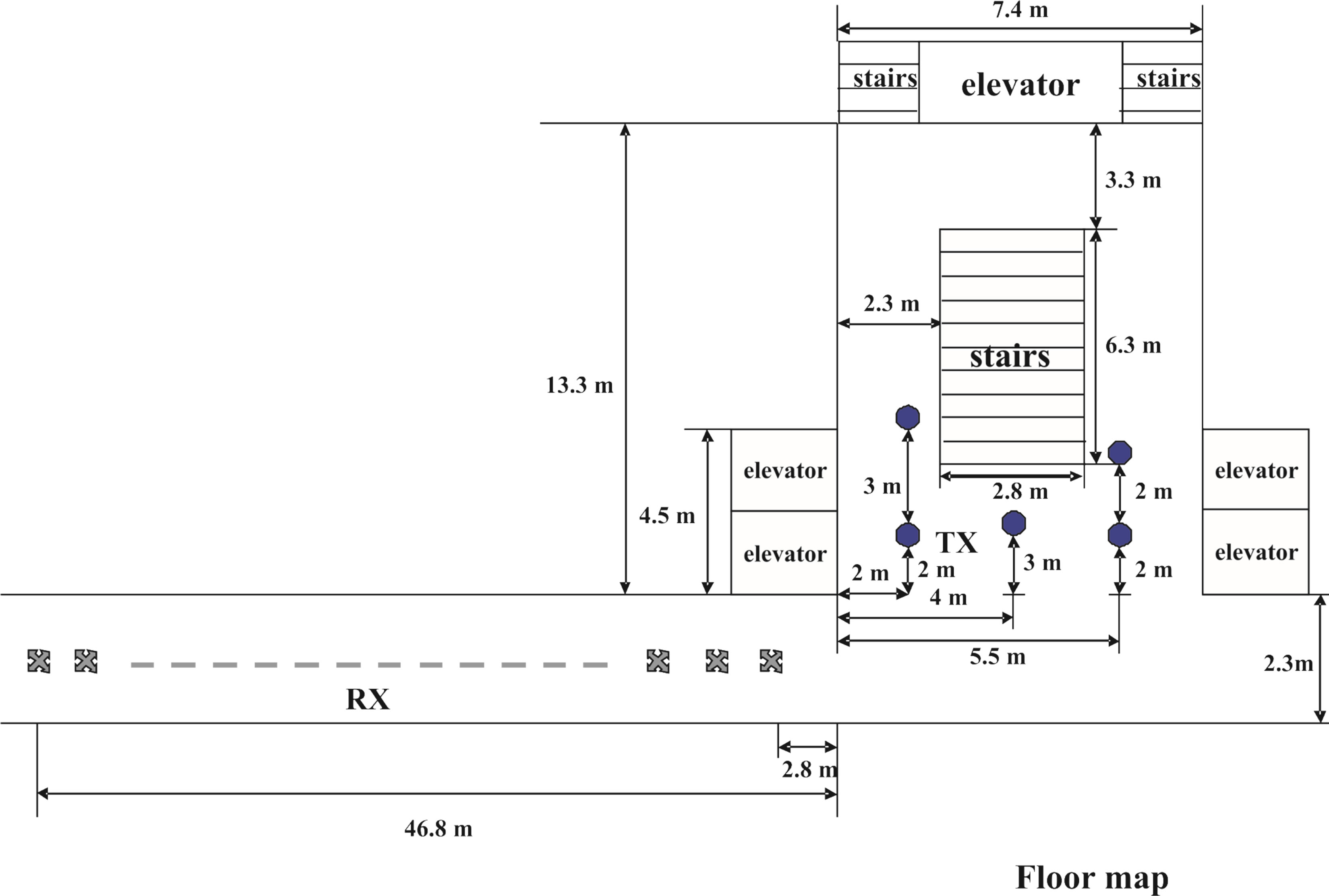
Figure 9. Measurement Setup: antennas are 0.9 m above the concrete floor. The measurements are done in the corridor of the Signals and Systems Group. The receiver is positioned at the left side of the corridor (i.e. the cross positions) and the transmitter is at the gray part as shown in the figure. The room contains one coffee machine, one garbage bin and one glass cabin.
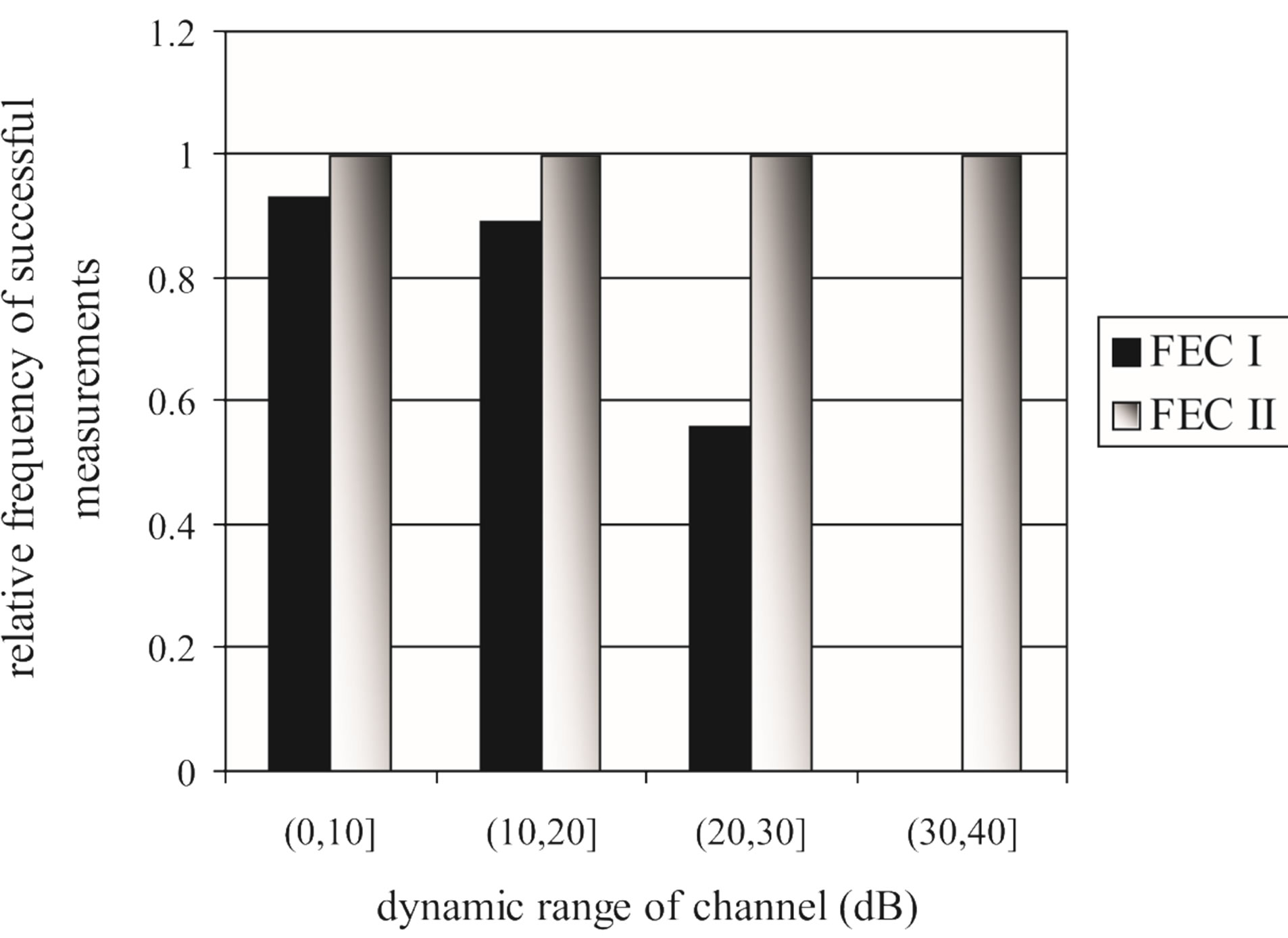
Figure 10. The comparison between FEC I and FEC II in the probability of successful measurements for each  range over 89 measurements. For FEC I, successful measurement means
 . For FEC II, measurement succeeds only if it has the error-free quality.
urements.
Here, we define  as the minimum SNR for FECI to achieve a BER of
  or lower and
  as the minimum SNR for FEC II to have the error-free quality for each measurement. The difference between
  and
and  is expressed as:
 (16)
(16)
If  (i.e.
(i.e. ), FEC I needs higher SNR (i.e. lower level of noise floor) to achieve
  than FEC II at BER = 0.
  is for the opposite case.
Figure 11 shows the statistical characteristics of ,
, and
and  at
at  and
and  dB, respectively.
• In the case of  dB, around 80% of
  is in the range of [10,12] dB and around 85% of
  is in the range of [9,10] dB, as shown in Figure 11(a). That already presents that FEC II needs lower SNR to have BER = 0 than FEC I to reach
 . Figure 11(b) shows whether
  is always larger than
  in every measurement at
  dB. Around 15% of measurements have the same SNR for both FEC I and II to reach their required BER. For the other 85% of measurements,
  is larger than
 . Their difference in around 50% of measurements is about 1 dB. On average,
  is around 11.4 dB,
  is around 9.9 dB and
  is around 1.5 dB. With
 , the average BER of FEC I is around
 . That concludes FEC II has a SNR gain of around 1.5 dB to reach the error-free quality comparing to FEC I at
  at
at  dB.
dB.
• In the case of  dB, both
  and
and  have a wider range with respect to
  dB, as we can see in Figure 11(a). Around 67% of
 is in the range of [11,16] dB while around 87% of
  lies in the same range. Figure 11(b) shows that
  is also not smaller than
  in the measurements at
  dB. Around 16% of measurements have the same SNR for FEC I and II to have successful measurements. In those 31 measurements at
  dB, the average
  is around 15 dB, the average
  is around 13.3 dB and their average difference
  is around 1.7 dB. With
  in Figure 11(a), the average BER of FEC I is around
 . Therefore, we can conclude that FEC II has a SNR gain of around 1.7 dB to have BER = 0 in comparison with FEC I to reach
  at
at  dB.
dB.
• In the case of  dB,
dB,  and
and  have different range to have successful measurements.
  lies in the range of [16,18] dB while
 is in the range of [12,15] dB. That means that FEC I always needs a higher SNR to achieve a BER of
  or lower than FEC II to have the error free quality. On average,
  is around 17.4 dB,
 is around 13.6 dB and
  is around 3.8 dB. In addition, the average BER of FEC I is around
  With
With . For the measurements at
  dB, we can say that FEC II has a SNR gain of around 3.8 dB to have no bit errors with respect to FEC I at
 .
.
As mentioned earlier, FEC I fails in the measurement at  dB but FEC II survives. By adding extra white noise, FEC II still have the error-free quality at SNR = 14dB. In general, FEC II performs better than FEC I in practice. To have successful measurement, their minimum SNR difference
  becomes larger as
  increases. That is also shown in the simulation.
6. Conclusions
Opportunistic error correction based on erasure codes is especially beneficial for OFDM systems to have an energy-efficient receiver. The key idea is to lower the dynamic range of the channel by a discarding part of the channel with deep fading. By transmitting one packet over a single sub-channel, erasure codes can reconstruct the original file by only using the packets transmitted over the sub-channels with high energy. Correspondingly, the wireless channel can have wire-like quality with the high mean and low dynamic range, leading to an increase of the noise floor. Correspondingly, the power consumption of wireless receivers can be reduced.
Opportunistic error correction consists of erasure codes and error correction codes. In this paper, we choose LT codes to encode source packets; then, each fountain-encoded packet is protected by the (175,255) LDPC code plus 7-bit CRC. To investigate the performance difference between the joint coding scheme (i.e. the LDPC code from the IEEE 802.11n standard) and this cross coding scheme, we compare them over the TG n channel with different dynamic range  in the simulation under the condition of the same code rate. Opportunistic error correction performs better in the simulation than the joint coding scheme if
  dB. Their performance difference becomes larger as
  increases. Besides, the performance of the joint coding scheme mainly depends on
 . When
  dB, opportunistic error correction does not have any performance loss as
  increases. Furthermore, we compare them in the experimental communication test bed. Measurement results show that opportunistic error correction works better than the joint coding scheme in any range of
 . In other words, this cross coding scheme is more robust to the imperfections of the practical systems.
7. Acknowledgements
The authors acknowledge the Dutch Ministry of Economic Affairs under the IOP Generic Communication— Senter Novem Program for the financial support.
NOTES
2In this paper, SNR is equivalent to Carrier-to-Noise Ratio.
3The TGn channel model is used by the High Throughput Task Group [20]. “TG” stands for Task Group and “n” stands for the IEEE 802.11n standard.
4 , where
  is the effective code rate (i.e. 0.5),
  is the code rate of LT codes (i.e.
 ) and
) and  is the code rate of the (175,255) LDPC code with 7-bit CRC (i.e.
 ).
).
5ADLINK, 80 MB/s High-Speed 32-CH Digital I/O PCI Card.
6AnalogDevices, 10-Bit, 40 MSPS, dual Transmit D/A Converter.
7Analog Devices, 2.5 GHz Direct Conversion Quadrature Modulator.
8Analog Devices, 800 MHz to 2.7 GHz RF/IF Quadrature Demodulator.
9AnalogDevices, Dual 12-Bit, 20/40/65 MSPS, 3V A/D Converter.
10The choice for QPSK instead of QAM-16 in the measurements is due to the noise floor of the testbed, whose noise floor is around -20 dB (i.e.  dB). Figure 6 shows that the required SNR for
  dB should be at least 20 dB for FEC I to achieve a BER of
  or lower. With the non-perfect synchronization and channel estimation, a higher SNR is expected in the real world than in the simulation to achieve the same order of BER. Therefore, we choose a lower order of modulation scheme to have more successful measurements to compare FEC I and II in the real world.