Journal of Applied Mathematics and Physics
Vol.05 No.01(2017), Article ID:73862,16 pages
10.4236/jamp.2017.51015
Reaction Mechanics for Point Objects
Philipp Kornreich1,2
11090 Wien, Austria
2King of Prussia, PA 19406, USA

Copyright © 2017 by author and Scientific Research Publishing Inc.
This work is licensed under the Creative Commons Attribution International License (CC BY 4.0).
http://creativecommons.org/licenses/by/4.0/


Received: December 5, 2016; Accepted: January 22, 2017; Published: January 25, 2017
ABSTRACT
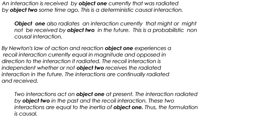
The least action principle is used to derive a general mathematical model of the motion of point objects subject to non-instantaneous interactions. A Lagrangian Equation of Motion, a Hamiltonian Formalism, a Poisson Bracket and the Relation of Reaction Mechanics and the General Theory of Relativity are derived here. In the limit of no delay, the equation of motion reverts to Newtonian Mechanics. In the limit of infinitesimal delay, the equation of motion takes the form of the Geodesic Equation of Motion of the General Theory of Relativity. For two objects, the single instantaneous interaction splits into two interactions when the propagation delay is considered. Object ONE experiences the following interactions at the present: it senses an interaction radiated by object TWO in the past. It also radiates an interaction that other objects might or might not sense in the future. It experiences a Recoil interaction equal in magnitude and opposed to the direction of the interaction it radiated. The Recoil interaction is independent of the radiated interaction reaching its target or not reaching its target. The Recoil interaction is causal.
Keywords:
Lagrangian, Hamiltonian, Poisson Bracket, Variational Method, Propagation Delay, Causal, Classical Mechanics, General Theory of Relativity

1. Introduction
Reaction Mechanics, a Mathematical Model of nature for systems of discrete point objects that takes non-instantaneous interactions into account is derived here. A Hamiltonian Formulism of Reaction Mechanics, the Reaction Mechanics Formulation of the Poison Bracket and the Relation of Reaction Mechanics and the General Theory of Relativity are derived here. In the limit of infinitesimal delay Reaction Mechanics reverts to the Geodesic Equation of Motion of the General Theory of Relativity. In the limit of no delay Reaction Mechanics reverts to Classical Mechanics.
The derivation is based on the most successful Mathematical Model of nature, Newtonian Mechanics [1] . Reaction Mechanics is also consistent with Special Relativity.
In the General Theory of Relativity [2] model of nature, a moving mass causes a disturbance of the space to propagate with the speed of light through the deformed space surrounding a mass. In the Electromagnetic Maxwell Model [3] a moving charge causes a disturbance to propagate with the speed of light through the electromagnetic field surrounding the charged object. The radiated disturbance in the space or field propagates in all directions. In the above models, a moving object experiences a Recoil interaction due to it radiating a disturbance in the space or field, see Figure 1. The Recoil interaction is independent of the future encounters of the radiated disturbance.
But this effect is not usually included when the interaction of two objects is calculated.
In the model of a propagating interaction, it is assumed that the objects are sufficiently far apart so that the disturbances in the space or field can be approximated by an interaction propagating between objects. In this case:
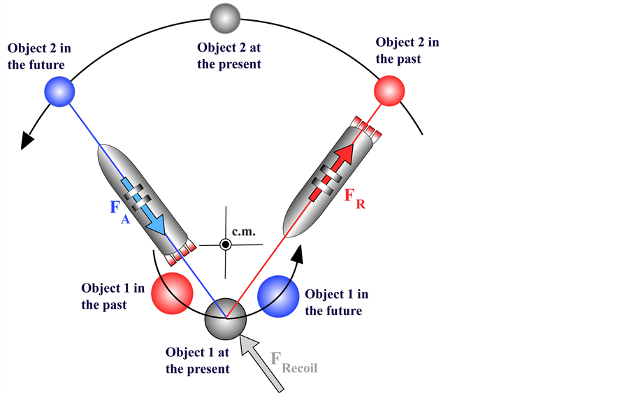
Figure 1. The forces act in directions opposed to the directions they propagate. The flight direction of the rockets symbolizes the direction of propagation of the interactions. The arrows symbolize the direction of the forces. Object 2 in the past radiated a force that reaches Object 1 at Present. Object 1 at present radiates a force that Object 2 might or might not sense at sometime in the future. By Newton’s law of action and reaction Object 1 at present experiences a Recoil force because it radiated the force . The Recoil force is equal in magnitude and opposed in direction to the force that Object 1 currently radiated. Thus, the interactions are causal.
The least action principle [1] in combination with the discrete Nagumo equation [4] is used to derive this mathematical model. In the limit of no delay the equation of motion derived here reverts to the Newtonian equation of motion. It is interesting to note that before reaching this limit, for infinitesimal delays this equation of motion reverts to the Geodesic Equation of Motion of the General Theory of Relativity [2] .
Often the interactions propagate with the speed of light. This effect is small and thus is often neglected. The single interaction between two objects in a model that considers interactions to be instantaneous is split into two interactions in a model that considers interactions which propagate with a finite velocity, see Figure 2.
When the interactions propagate with the velocity of light between objects the model is consistent with special relativity. Unfortunately, it is the future interac-
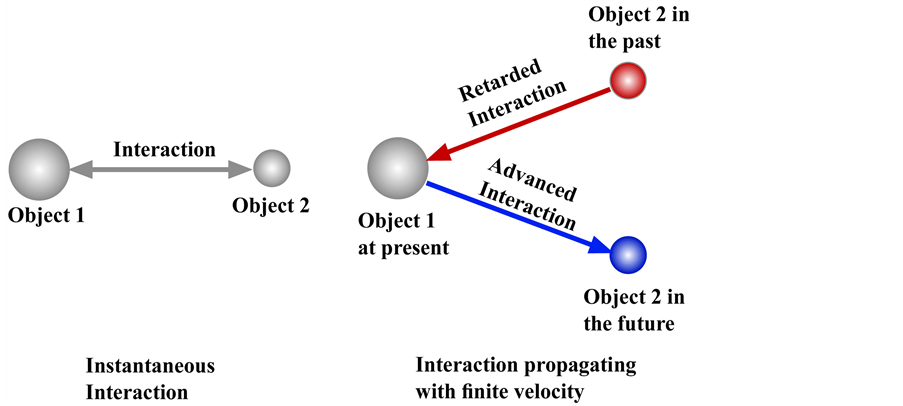
Figure 2. The interaction propagating with a finite velocity between objects removes some of the spatial symmetry. This splits the single instantaneous interaction into two interactions for the case of an interaction propagating with a finite velocity. This preserves time inversion symmetry.
tion, the Advanced interaction, that appears in the mathematical formulation instead of an explicit Recoil interaction. This formulation preserves time inversion symmetry. Only the Retarded interaction radiated by another object in the past and the Recoil interaction act currently on an object. The Advanced interaction which an object radiates does not act on the radiating object.
In the orbital model of pairs of point objects coupled by an instantaneous interaction the orbital and center of mass motions are independent. In the case where the interactions take time to propagate between objects this symmetry is removed. The removal of this symmetry couples the orbital and center of mass motions. Energy and angular momentum are transferred between these modes of the motion [5] . The total energy and momentum are conserved.
When the orbit of two objects around each other is eccentric, the propagation time of the interaction between the objects changes periodically. The periodic change in the delayed interaction of the orbital motion pumps the center of mass motion. It is similar to increasing the motion of a swing by periodically pushing it. This transfers energy and angular momentum from the orbital motion to the center of mass motion. The angular momentum of the center of mass motion increases with time. Therefore, the center of mass accelerates [5] .
S. Carlip [6] , I J. Good [7] , and A. P. Lightman et al. [8] , state: “It is certainly true, although perhaps not widely enough appreciated, that observations are incompatible with Newtonian gravity with a light-speed propagation delay added in. .... it is known that Solar System orbits would shift substantially on a time scale on the order of a hundred years.” The calculations that led to this erroneous conclusion only used the retarded part of the interaction.
The problem of interactions that propagate with a finite velocity has been discussed by many eminent scientists. They consider both the Retarded and Advanced parts of the interaction. Carl Friedrich Gauss [9] in 1845 was the first scientist recorded to discuss interactions at a distance that propagate with a finite velocity. Others were K. Schwarzschild [10] , W. Ritz (1908), H. Tetrode [11] (1922), A. D. Fokker [12] (1929), J. H. Wheeler, R. Feynman [13] (1945), R. V. Kamat [14] (1970), K and M Imaeda (1982), etc.
Advanced and retarded interactions have been discussed in Electromagnetic Theory texts. Most electromagnetic texts [3] [15] [16] only consider the causal retarded part of the interaction. Panofsky and Phillips [16] do mention an advanced interaction but discard it on the grounds that it is non causal.
Indeed the example of a charged particle is the most often discussed problem involving advanced and retarded interactions. Paul A. M. Dirac [17] (1938) gives a model for explaining the forces on an accelerating charged particle. John Archibald Wheeler and Richard Feynman [13] postulated a so called “Absorber Theory” of Radiation. They do take both advanced and retarded interactions into consideration. They acknowledge that Hugo Martin Tetrode [11] was the first to introduce the concept of an Absorber. Tetrode also stated that the sun would not radiate if it were alone in space since no other bodies could absorb its radiation. Tetrode also believed that the atoms from a star knew 100 years ago that the light which the star radiated would interact with his eyes 100 years later.
Wheeler and Feynman [13] postulate similarly to Tetrode’s [11] ideas that:
1) A charged accelerating particle does not radiate in the absence of other charges.
2) The fields acting on a given charge arise only from other charges.
3) These fields are equal to one half the retarded plus one half the advanced solution of Maxwell’s equations. This law of forces is symmetric with respect to past and future.
4) Sufficiently many particles are present to absorb completely the radiation given off by the source. This is the “Absorber” postulate.
The concept presented here of a Recoil interaction equal in magnitude and opposite in direction to the Advanced interaction, eliminates the need for concepts listed in 1, 2, and 4. Tetrode’s star did not need to know what its light will illuminate 100 years later, because the Recoil interaction is independent of the Advanced interaction reaching its target or not reaching its target.
Alfred Lande [18] wrote a short critique of Wheeler and Feynman’s Absorption Theory [13] . He too, does not agree with the concept that the atoms of a star knew 100 years ago that the light will interact currently with an observer’s eyes. He also disagreed that an Absorber is necessary to explain the forces acting on an accelerating particle.
Reaction Mechanics does not require an Absorber or need objects to know whether or not the interactions they radiate will reach its destination.
A Reaction Mechanical extension of Classical Mechanics is derived here. However, it would be interesting to extend this Mathematical Model to the Quantum Mechanical regime.
2. Equation of Motion of Reaction Mechanics
In order to derive the Mathematical Model of Reaction Mechanics for systems of discrete point objects a causal Lagrangian is postulated. It is a function of; the present coordinate vector with components at an arbitrarily defined universal time , of the present velocity vector with components at time , a past coordinate vector with components at time , and a past velocity vector with components at time . The coordinates and velocities have to be specified with respect to an inertial coordinate frame. The time differences, for example between times and , differ by more than infinitesimal quantities. The time differences represent the propagation times of the interactions. The coordinates do not necessarily need to be position vectors. They can be more generalized quantities and can have any number of dimensions.
In special-relativity, the objects are located by four dimensional coordinates , where . Here , c is the velocity of light in free space and is the time. In special-relativistic cases, the time is not a pre-determined parameter in terms of which the position vectors are calculated. In the special-relativistic case the time is a variable similar to the components of the position vector. Here the velocity of light c is a constant. In special-relativity, the four dimensional space is flat. But all position and time components are functions of a parameter . The calculations have to be performed subject to the Constraint that the velocity of light is constant. This is described by H Minkovski in the chapter “Space and Time” in reference [2] . The components of the generalized velocity vector and the components of the generalized acceleration vector are:
(1)
where τ is an arbitrarily defined universal time. In Classical Mechanics problems τ becomes the time t. In the case of the Special Relativity τ becomes a parameter in terms of which the four vector components are calculated.
A method similar to the Hamiltonian method is followed for deriving the equation of motion of Reaction Mechanics. In this paper, in order to include the effect of both finite and infinitesimal time increments in the derivation of the equation of motion a sum S of Lagrangians is used. This is similar to the discrete Nagumo equation [4] .
(2)
The sum S contains terms that occurred in the past, that occur currently, and terms that might occur in the future. The terms occurring in the past and currently are causal and deterministic. For the purpose of this derivation the future coordinates are treated the same as the past coordinates. The real physical significance of the future terms will be explained near the end of this chapter. It eventually will be shown that the non causal future terms are equal to causal deterministic terms. But at this point of the discussion, the past, current and future terms are treated equally.
In order to derive an equation of motion an action integral I is formulated.
(3)
It is assumed that the Lagrangians, their first and second derivatives with respect to the coordinate and velocity components are continuous in the interval to . The calculus of variation will be used for determining a relation among the coordinate components for which the action integral I has an extremum value.
In this process one can also include Constraints . The Constraints are limited to a type for which a sum Z can be formed.
(4)
and where the sum Z of constraints is equal to a sum of constants .
(5)
Since Equation (5) is equal to zero it can be multiplied by a constant, , a Lagrange multiplier, and added to the action integral of Equation (3) without changing it.
(6)
It is, of course possible to have more than one constraint. Here the subscript j labels the particular constraints. By substituting Equations (2), (4) and (5) for the sum of Lagrangians and the sum of constraints into the action integral of equation 6 one obtains:
#Math_45# (7)
where dummy variables are introduced so that one can vary the coordinate components to obtain an optimum path. The path through the multi dimensional space defined by these coordinates will be optimum if all the changes of the action integral with each dummy variable is zero.
(8)
This includes points where the action integral is a maximum with respect to some dummy variables and a minimum with respect to other dummy variables. There may be saddle points in the equation. By substituting Equation (7) into Equation (8) one obtains:
(9)
where summation over repeated Greek indices is used. Note that only the Lagrangian and and Constraints and contain the current coordinate vector components and the current velocity vector components . No other Lagrangian or Constraint contains the current coordinate vector components and the current velocity vector components . The various Constraints in Equation (9) are labeled by j. Equation (9) can be integrated by parts:
(10)
It is assumed that all the variations of the coordinates with the dummy variables , go to zero at the limits of integration and Also, the fundamental lemma of the Calculus of Variation states that since the variation of the coordinates with the dummy variables , are arbi-
trary, the integrals will go to zero if the square brackets are equal to zero. This yields the following Euler Lagrange equation of motion:
(11)
Equation (11) is a combination of the conventional Euler Lagrange equation and the discrete Nagumo equation. The Lagrange multipliers have to be evaluated by substituting the coordinate components calculated from the equation of motion, Equation (11), into the constraint equations, Equation (5). Here is a function of the current and the past coordinates and velocities while is a function of the current and future coordinates and velocities.
(12)
Equation (11) is the Equation of Motion of Reaction Mechanics. Equation (11) represents three equations in Classical Mechanics. In the case of Special Relativity Equation (11) represents four parametric equations. In the case of Special Relativity the Constraint that the velocity of light is constant has to be included. This equation describes the development of the current coordinates of a particular object. It contains retarded, current and apparent advanced terms. As discussed previously the retarded terms are interpreted as interactions acting on the system currently that were radiated by other parts of the system previously, at points specified by the retarded coordinates. These are deterministic and causal interactions. The apparent future coordinates appearing in Equation (11) are actually a description of the Recoil interaction. The Recoil interaction occurs currently but is described in terms of current and apparent future coordinates. This formulation preserves time inversion symmetry. The true future Advanced interaction does not appear in Equation (11). It does not act on the object whose motion is described by Equation (11).
In summary, each object experiences two interactions. One interaction was radiated by other objects in the past and a Recoil interaction due to this object also radiating an interaction currently. These two interactions are equal to the inertia of the object under discussion. The interactions are causal.
With this definition both the retarded and advanced terms are causal deterministic interactions. The fact that in the formulation, the future coordinates appearing in the Recoil term is a mathematical peculiarity, physically all events occur in causal order.
In this mathematical model it is necessary to know some features of the point objects of the system over a span of time so that causal Lagrangians can be formulated. In order to obtain a solution of the equation of motion, Equation (11), initial conditions will have to be specified. In this case it is required that one not only specify the values of the coordinates and their derivatives at an instant of time but specify the coordinates and their derivatives over a continuous range of time.
3. Relation to the General Relativity Theory
In the limit of zero delay the mathematical model of Reaction Mechanics reverts to Newtonian Mechanics. That is, Equation (11) reverts to the Euler Lagrange equation of Classical Mechanics. In the limit of infinitesimal delay Equation (11) of Reaction Mechanics reverts to the geodesic equation of motion of the General Theory of Relativity.
Next, this connection between Reaction Mechanics and the General Theory of Relativity is investigated. The geodesic equation of motion in a curved space as used in the General Theory of Relativity is derived in §9 of the chapter titled “The Foundations of the General Theory of Relativity” by A. Einstein in the book “The Principle of Relativity” by A Einstein, H. A. Lorentz, H. Weyl and H. Minkowski [2] . The geodesic equation of motion is obtained by substituting equation 20c into equation 20b on page 132 with ω set equal to one. The resulting equation is:
(13)
Summation over repeated Greek indices is used. Here is an element of the geodesic tensor. The Euler Lagrange equation of Classical Mechanics, the geodesic equation of motion of the General Theory of Relativity, Equation (13), and the equation of motion of Reaction Mechanics, Equation (11), are all derived by the same variational method. The geodesic tensor is used to specify the length of a distance element dρ in the curved four dimensional space as used in this relativistic model.
(14)
Light follows the curvature of space. Since people perceive light as going straight, this results in people seeing a distorted picture. An example of this can be seen by observing a star as it is being eclipsed by the sun moving in front of it. As the light ray from the star to our eyes passes closer and closer to the sun it is bent more. But since people perceive light as going straight one sees the star moving farther and closer to the sun.
By rewriting the second term of Equation (13) and multiplying by the inverse geodesic tensor with components one obtains the equation of motion of the geodesic tensor:
(15)
where is a component of the Christoffel symbol of the second kind defined as:
(16)
Here is a component of the inverse of the geodesic tensor. A very good description of Tensor Calculus is given in “The Principle of Relativity” By A Einstein, H. A. Lorentz, H. Weyl and H. Minkowski [2] .
The General Theory of Relativity also reverts to Newtonian Mechanics in the limit of the absence of gravitational and other potentials. The absence of gravitational and other potentials results in a flat space. In this case the geodesic tensor is diagonal and constant. This leaves only the acceleration equal to zero in Equation (15) in agreement with Newtonian Mechanics.
Both Newtonian Mechanics and the General Theory of Relativity describe the motion of classical systems under different assumptions. Therefore, Reaction Mechanics in some limit must give the same description as the General Theory of Relativity. This is, of course, true in the limit of the absence of all potentials delayed or otherwise. However, in the limit of very small delay times θ, the equation of motion of Reaction Mechanics assumes the form of the geodesic equation of motion of the General Theory of Relativity, Equation (15). This can be demonstrated as follows:
The equation of motion of Reaction Mechanics, Equation (11) without constraints and where it is assumed that the coordinates have four components as conventionally used in the relativistic case, with is:
(17)
As described before, objects are located at different four dimensional coordinates . Consider the case where the Lagrangian is a function of the current and past coordinate components, and the current and past velocity components. Therefore, the Lagrangian is a function of the current and future coordinate components and the current and future velocity components. For small delay times θ, one can expand the sum of Lagrangians to second order:
#Math_84# (18)
where summation over repeated indices is implied. The last term of Equation (18) is a higher order term which has been neglected. Here the zero order Lagrangian is:
(19)
One can define a covarient second rank tensor with components :
(20)
This tensor with components is symmetric. The components of the tensor have dimensions of mass. By substituting Equation (20) into Equation (18b) and the resulting expression into the equation of motion, Equation (17) one obtains:
(21)
Using the chain rule for the general time derivative of the second rank tensor elements one obtains:
(22)
The first two terms are the Euler Lagrange equation of Classical Mechanics operating on the zero order Lagrangian and therefore must be equal to zero. This is consistent if one considers Newtonian Classical Mechanics, the General Theory of Relativity and Reaction Mechanics as approximate mathematical models that describe how nature functions. Thus, all these mathematical models can coexist. The motions described by each theory give results that approximate nature to a certain accuracy. This leaves:
(23)
where the forth term of Equation (22) has been expanded similarly to Equations (13) and (15). By multiplying Equation (23) by the inverse tensor with components one obtains an equation identical to the geodesic tenser equation of motion, Equation (15), of the General Theory of Relativity.
(24)
where the components of the Christoffel symbol of the second kind are:
(25)
The components of the tensor are proportional to the elements of the geodesic tensor.
(26)
Here an infinitesimal distance is:
(27)
where C is a constant with dimension of reciprocal mass. Thus, in the limit of infinitesimal delay the equation of motion of Reaction Mechanics takes the form of the geodesic tensor equation of motion of the General Theory of Relativity, Equation (15). If the second derivative of the Lagrangian potential and the delay time θ are large, then the second rank tensor with components will be large. The larger the second rank tensor with components the larger the distortion of the space.
The geodesic equation of motion, Equation (24), can be used in the conventional way for the Rimann Christoffel tensor with components - in the Einstein Field Equation [19] [20] of the General Theory of Relativity.
(28)
where is a component of the Einstein Tensor which is a function of the Christoffel symbols, is the gravitational constant, c is the speed of light in vacuum, is the cosmological constant and is a component of the stress energy tensor. Where is given by:
(29)
The tensor Equation (28) together with Equation (29) result in ten equations for the ten components of the symmetric geodesic tensor. The components of the geodesic tensor describe the curvature of the space resulting from the presence of masses and energy. A more detailed derivation of Equation (29a) is given in §12 of the chapter titled “The Foundations of the General Theory of Relativity” by A. Einstein of reference [2] .
Consider the example of a three dimensional, invers distance, centrally symmetric potential. The Lagrangian and the delay parameter θ have the following form in this case:
(30)
where m is a test mass, is a component of the test mass position vector, is a component of the test mass velocity vector, M is a stationary mass located at the origin of an inertial coordinate system and G is the gravitational constant. By substituting Equation (30) into Equation (20) one obtains for the six components of the second rank tensor given by Equation (20).
(31)
where the Schwarzschild radius of the stationary mass M is given by:
(32)
The corresponding geodesic tensor components are given by Equation (26). The second rank tensor for ν ≠ 4, α ≠ 4 is very small for distances substantially outside the Schwarzschild radius. Thus for the three dimensional inverse distance potential only the component can have a significant value at distances outside the Schwarzschild radius. This is in agreement with the assumption made for the derivation of the inverse distance potential of Newton’s equation from the equation of motion of the General Theory of Relativity. This derivation is performed in §21 titled “Newton’s Theory as a First Approximation” of the chapter titled “The Foundation of the General Theory of Relativity” by A. Einstein of reference [2] . Recall that the derivation performed in equations 30 and 31 started with an inverse distance potential. Thus, this derivation is self consistent.
In the volume near the Schwarzschild radius Newtonian Mechanics does not hold. In this volume one needs to consider the curvature of space.
4. Hamiltonian Reaction Mechanics Equation of Motion and the Poison Bracket
The Hamiltonian is a function of the momentum vector components and position vector components. Thus one needs to define a momentum with components at the present time, at time step as follows:
(33)
By substituting Equation (2) for the sum of Lagrangians into Equation (33) one obtains for the momentum components:
(34)
Observe that the momentum is a function of the retarded, present and advanced coordinates and velocity components . Thus, the momentum with components of the non local interactions includes both the momentum of the point objects as well as the momentum of an interaction field.
The Hamiltonian sum H is the Legender transform of the sum S of Lagrangians with respect to all the velocity vector components.
(35)
Since the sum of Lagrangians S is a function of all the position vector components and velocity vector components the change dS in the sum of Lagrangians can be written as:
(36)
From Equation (35) the change in the Hamiltonian sum H is:
(37)
By substituting Equation (36) into Equation (37) and making use of Equations (11) with the constraints set equal to zero one obtains:
(38)
By collecting terms one obtains:
(39)
This shows that the Hamiltonian sum is a function of the ’s and ’s. Thus, the change of the Hamiltonian sum can be written as:
(40)
By comparing Equations (39) and (40) one obtains the Hamiltonian equations of motion of Reaction Mechanics:
(41)
It is useful to investigate the derivative of the Hamiltonian with respect to an arbitrarily defined universal time τ. One obtains by calculating the time derivative of Equation (35)
(42)
By using Equation (33) in Equation (42) and collecting terms one obtains:
(43)
Therefore, when the time rate of change of the momentum is equal to the generalized force of the problem, the Hamiltonian is a constant of the motion.
Next, consider the time derivative of some quantity
(44)
By substituting Equation (41) into Equation (44) one obtains Poisson Bracket of Reaction Mechanics.
(45)
Note that it is the Hamiltonian sum that appears in the Reaction Mechanics Hamiltonian equation of motion. Also the momentum appearing in these equations is a sum. The Momentum contains features of the interaction field.
5. Conclusions
A mathematical model of nature for interactions that propagate with a finite velocity was presented in here. The propagations take time and thus are not instantaneous. An equation of motion for systems of discrete point objects that are subject to non-instantaneous interactions is derived here. The least action principle in combination with the discrete Nagumo equation was used for this derivation. An equation of motion of Reaction Mechanics, the form of the momentum, a Hamiltonian Formalism and Poisson Bracket for systems with delayed interactions, and the relation of Reaction Mechanics and the General Theory of Relativity were obtained here. In the limit of no delay the equation of motion of Reaction Mechanics reverts to the equation of motion of Newtonian Mechanics. In the limit of infinitesimal delay, the equation of motion takes the form of the geodesic tensor equation of motion of the General Theory of Relativity. The equation of motion is a combination of a continuous variable differential equation and a difference equation.
The equation of motion generates retarded and advanced terms from a sum of causal Lagrangians. This preserves time inversion symmetry. The retarded terms in the equation of motion describe interactions sensed by a point object at the present that were radiated by some other objects in the past. This interaction is causal. The point object, also, radiates an interaction that might or might not be sensed by other objects in the future. The point object by radiating an interaction experiences a Recoil interaction. The Recoil interaction is causal. The interaction which the point object radiated has no effect on the point object. Also, the Recoil interaction is independent of the radiated interaction reaching its target or not reaching its target. The point object experiences two interactions, one radiated by other objects in the past and the Recoil interaction. These interactions are equal to the inertia of the object. Thus, the delayed interactions are causal.
The equations obtained here are derived from the most successful mathematical model of nature, Newtonian Mechanics.
Acknowledgements
I thank my wife Marlene for our discussions about the subject matter of this paper. I also thank her for proof reading, for correcting my mistakes and for her assistance in the formulating of this paper.
Cite this paper
Kornreich, P. (2017) Reaction Mechanics for Point Objects. Journal of Applied Mathematics and Physics, 5, 137-152. http://dx.doi.org/10.4236/jamp.2017.51015
References
- 1. Herbert, G. (1980) Classical Mechanics. Addison-Wesley Publishing Company, Reading, MA.
- 2. Einstein, A., Lorentz, H.A., Weyl, H. and Minkowski, H. (Republished 1952, Originally Translated in 1923) The Principles of Relativity. Dover Publishing Co., New York.
- 3. Jackson John Paul (1962) Classical Electrodynamics. John Wiley and Sons Inc., New York, London, Library of Congress No. 62-8774.
- 4. Chow, S. and Shen, W. (1995) Dynamics in a Discrete Nagumo Equation: Spatial Topological Chaos. Journal of Applied Mathematics, 55, 1764-1781. https://doi.org/10.1137/s0036139994261757
- 5. Philipp, K. (2016) The Contribution of the Gravitational Propagation Delay to the Orbital and Center of Mass Motions. The Journal of Modern Physics, Online.
- 6. Carlip, S. (2000) Aberration and the Speed of Gravity. Physics Letters, A267, 81-87. https://doi.org/10.1016/S0375-9601(00)00101-8
- 7. Good, I.J. (1975) Infinite Speed of Propagation of Gravitation in Newtonian Physics. American Journal of Physics, 43, 640-641. https://doi.org/10.1119/1.9766
- 8. Lightman, A.P., Press, W.H., Price, R.H. and Teukolsky, S.A. (1975) Concepts of Mass in Contemporary Physics and Philosophy. Problem Book in Relativity and Gravitation, Princeton University Press, Princeton.
- 9. Gauss Carl Friedrich to Weber Wilhelm 19 March 1845, Gauss Weber 5:627-29 esp. 629; Weber to Gauss 31 March 1845 Niedersächsische Staatsund Universitätsbibliothek Göttingen, Gauss Nachla&beta Nr. 31 1945 and published in Wiederkehr, “Wilhelm Weber Stellung” 68, see also Kaiser, “Theorien der Elektrodynamy” 109.
- 10. Schwarzschild, K. (1916) über das Gravitationsfeld eines Massenpunktes Nach dereinsteinischen Theori. Sitzungsberichte der Deutschen Akademie der Wissenschaften zu Berlin Klasse für Mathematik, Physik und Technik, 189.
- 11. Tetrode, H. (1922) über den Wirkungszusammenhang der Welt. Eine Erweiterung der klassischen Dynamik. Zeitschrift fur Physik, 10, 317-328. https://doi.org/10.1007/BF01332574
- 12. Fokker, A.D. (1929) Ein Invariante Variationssatz für die bewegung Mehrerer Elektrischer Massteilchen. Zeitschrift für Physik, 58, 386-393. https://doi.org/10.1007/BF01340389
- 13. Wheeler, J.A. and Feynman, R. (1945) Absorber Theory and the Radiation Arrow of Time. Review of Modern Physics, 17, 157-181. https://doi.org/10.1103/RevModPhys.17.157
- 14. Kamat, R.V. Action Principles of Physics.
- 15. Stratton, J. (1941) Electromagnetic Theory. John Wiley and Sons Inc., New York.
- 16. Panofsky Wolfgang, K.H. and Phillips, M. (1962) Classical Electricity and Magnetism. Addison-Wesley Publishing Company Inc., Upper Saddle River.
- 17. Dirac, P.A.M. (1938) Classical Theory of Radiating Electrons. Proceedings of the Royal Society of London A, 167, 148-169. https://doi.org/10.1098/rspa.1938.0124
- 18. Lande, A. (1950) On Advanced and Retarded Potentials. Physical Review, 80, 283. https://doi.org/10.1103/PhysRev.80.283
- 19. Einsteins Field Equations. https://en.wikipedia.org/wiki/Einstein_field_equation
- 20. Baez, J.C. and Bunn, E.F. The Meaning of Einstei’s Equation. University of California, Riverside. http://math.ucr.edu/home/baez/physics/