Open Journal of Fluid Dynamics
Vol.04 No.05(2014), Article ID:52861,8 pages
10.4236/ojfd.2014.45037
A Micromixer Using the Taylor-Dean Flow: Effect of Inflow Conditions on the Mixing
Toshihiko Kawabe1, Yasutaka Hayamizu2, Shinichiro Yanase3, Takeshi Gonda2, Shinichi Morita2, Shigeru Ohtsuka2, Kyoji Yamamoto3
1Technical Division, Tsurumi Manufacturing Co., Ltd., Tottori, Japan
2Department of Mechanical Engineering, Yonago National College of Technology, Tottori, Japan
3Graduate School of Natural Science and Technology, Okayama University, Okayama, Japan
Email: hayamizu@yonago-k.ac.jp
Copyright © 2014 by authors and Scientific Research Publishing Inc.
This work is licensed under the Creative Commons Attribution International License (CC BY).
http://creativecommons.org/licenses/by/4.0/


Received 30 October 2014; revised 24 November 2014; accepted 20 December 2014
ABSTRACT
Chaotic mixing in a curved-square channel flow is studied experimentally and numerically. Two walls of the channel (inner and top walls) rotate around the center of curvature and a pressure gradient is imposed in the direction toward the exit of the channel. This flow is a kind of Taylor- Dean flows. There are two parameters dominating the flow, the Dean number De (∝ the pressure gradient or the Reynolds number) and the Taylor number Tr (∝ the angular velocity of the wall rotation). In the present paper, we analyze the physical mechanism of chaotic mixing in the Taylor-Dean flow by comparing experimental and numerical results. We produced a micromixer model of the curved channel several centimeters long with square cross section of a few millimeters side. The secondary flow was measured using laser induced fluorescence (LIF) method to examine secondary flow characteristics. We also performed three-dimensional numerical simulations for the exactly same configuration as the experimental system to study the mechanism of chaotic mixing. It is found that good mixing performance is achieved for the case of De ≤ 0.1Tr, and that mixing efficiency changes according to the difference in inflow conditions. The flow is studied both experimentally and numerically, and both results agree with each other very well.
Keywords:
Taylor-Dean Flow, Chaotic Mixing, Secondary Flow, LIF, CFD

1. Introduction
Recently, great attention has been paid to the development of a micro-chemical-analysis device called the micro total analysis systems (μTAS) in the field of engineering. This device, which consists of various microflow devices and sensors, functions through a series of operations such as mixture, reaction, separation, and extraction. However, the flow is in the very low Reynolds number region because of the microsize of the channel, where mechanical mixing by turbulence cannot be expected without a special artifice. Currently, a micromixer is needed to mix low-Reynolds-number flows efficiently. Stroock et al. [1] studied a micromixer generating secondary flows in a channel by carving a ditch into the channel wall surface. Kim et al. [2] also studied a micromixer using a similar method. Sato et al. [3] made a micromixer that generates stronger secondary flows by carving ditches into the three wall surfaces of the channel. It has been shown that these methods are effective when the flow velocity is fast, although the pressure loss becomes a serious problem in this case.
On the other hand, a micromixer that uses chaos of the flow caused by a time-periodic perturbation was studied by Niu and Lee [4] and Tabeling et al. [5] . It was shown that the flow is miscible within a relatively short channel distance from the entrance compared with the mixing using only secondary flows.
We then proposed a micromixer making use of chaos of the secondary flow, specifically, a micromixer in which the secondary flow becomes chaotic through a curved channel where two walls of the channel rotate [6] . This flow is a kind of Taylor-Dean flows [7] . In the present paper, we analyze the physical mechanism of chaotic mixing in the rotating curved channel flow by comparing experimental and numerical results. The secondary flow was measured by laser induced fluorescence (LIF) method to examine secondary flow characteristics. We also performed three-dimensional numerical simulations for exactly the same configuration as the experimental setup to study the mechanism of chaotic mixing.
2. Experimental Methods
2.1. Experimental Setup
A diagram of the experimental setup is shown in Figure 1. Two working fluids (70 wt% of glycerol aqueous solution and 70 wt% of glycerol aqueous solution dissolving rhodamine B at the 2.5 ppm concentration) which are reserved in the tank ①, ② are drawn to the overflow tank ⑤, ⑥ by the pump ③, ④. Then, it flows into the curved channel, a test section ⑨, via the inlet tube ⑦ and goes to the drain tank. The test section consists of two parts, i.e., the rotor and the casing. The channel is formed of the casing and the rotor where the upper wall and right (inner) wall of the channel are the rotor walls capable of being rotated (refer to Figure 2) when one sees from the upstream of the entrance. The rotor is rotated by the motor ⑧. The flux of the test section can be controlled by the needle valve ⑩ which is at the exit of the test section. We measured the number of revolutions of the rotor and the weight of outflow of working fluid during a certain time. A viewing block ⑪ is installed to ease the refraction of light in case of visualization of the secondary flow. We used Davis8 (LaVision) for LIF.
2.2. Curved Channel and Method of Visualization
The dimension of the curved channel is shown in Table 1. Here,  is the width and height of the curved channel,
  the radius of curvature of the center line of the curved channel, and
  the total length of the channel. The nondimensional curvature
  is given by
 . (1)
. (1)
Other nondimensional parameters concerned are the Reynolds number Re, the Dean number De [8] and the Taylor number Tr [7] . These are given by
 , (2)
, (2)
 , (3)
, (3)
 , (4)
, (4)
where  is the flux of the curved channel,
  the kinematic viscosity, and
  the angular velocity of the rotor. If the rotation of the rotor is in the same direction as the mean flow in the channel, the parameter
  is taken to be positive; otherwise, it is negative.

Figure 1. Diagram of the experimental setup.
 (a)
(a)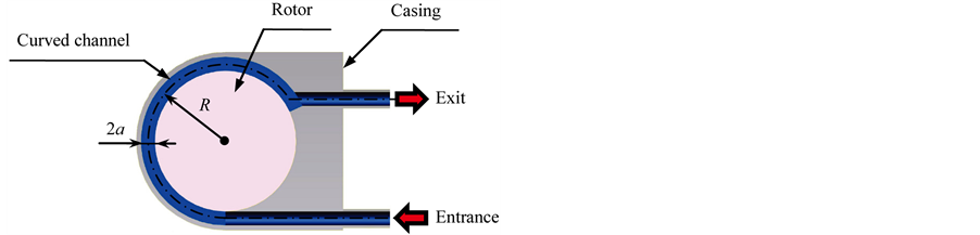 (b)
(b) (c)
(c)
Figure 2. Enlargement of the test section. (a) 3-D view of the test section; (b) Top view of the test section; (c) Cross section view of the test section.

Table 1. Dimension of the curved channel.
Next we explain the method of visualization of the flow. A scheme of the method of visualization is shown in Figure 3. The laser sheet lights up a cross section of the channel normal to the channel side wall and the photographs of the secondary flow patterns are taken by a high speed camera. Also, the photographs in a cross section at 180˚ downstream from the curved channel entrance are seen from the upstream.
We acquired the fluorescence only of the rhodamine B by installing the high-pass filter (transmitted wave length of 570 nm or more) in a high speed camera for LIF to calculate the concentration distribution. We also measured the viscosity of glycerol aqueous solution using the precision rotational viscometer before and after the experiment and confirmed that there was no change of viscosity throughout the experiment. The density of glycerol aqueous solution was calculated by use of the gravimeter.
3. Numerical Simulations Methods
To examine the secondary flow characteristics in detail, we also performed three-dimensional numerical simulations for exactly the same configuration as the experimental setup. We used OpenFOAM [9] for numerical simulations. The Navier-Stokes equations were solved using the icoFoam solver in which the PISO method is used for numerical calculations to obtain the flow configuration. As the inflow boundary condition, we imposed a constant axial velocity at the entrance of the channel. Constant value for the pressure and zero gradient for the velocity are imposed at the exit of the channel. After obtaining the velocity field, we solve the transport equation for the concentration using the scalarTransportFoam solver in which the SIMPLE method is used for the numerical calculation. The diffusivity is taken to be zero in the present calculation although the numerical diffusivity may be efficient in the present calculations. Two boundary conditions (refer to Figure 4) for the concentration distribution were applied at the entrance of the channel. Note that the right-hand side of each figure is the rotating inner wall.
4. Results and Discussion
4.1. Experimental Results
Figure 5 and Figure 6 show experimental results of LIF under the conditions I and II at the cross section of 180˚ downstream from the curved channel entrance. The right and top sides of each picture are moving walls that moves in the perpendicular direction to the sheet of the picture, while the left and bottom sides are stationary walls. The direction of the mean flow is to the other side of the sheet. Since the concentration of rhodamine B is 100% in the half side of the entrance and 0% in the other side, it is judged that mixing is promoted if the region with intermediate concentration between 100% and 0%, specifically 50%, increases.
When , the interface deformation can be observed as De increases for both conditions I and II; however, there is no change in concentration and the two are separate. Mixing itself is not facilitated. When
 , for conditions I and II, mixing is greatly facilitated in
  and 0.3, and the circa 50% concentration region grows. However, when De increases to 1.0, interface deformation can be observed; yet, as in
 , the respective fluid bodies are separate and mixing is scarcely facilitated. When
 , similar tendencies can be observed under both conditions, but it can be observed that the state of mixture differs greatly from the case of
 .
.
Therefore, the experimental results have shown that mixing is highly promoted around the range of  for both conditions. The condition of occurrence of mixing is expressed by
  whatever sign of Tr is (the direction of the rotation of rotor is the same of the mean flow or the reverse). However, the sign of Tr gives a strong influence on the way of mixing, specifically in the spatial structure.
4.2. Numerical Simulations Results
Figure 7 and Figure 8 show the results of the numerical simulations using OpenFOAM. As the experimental results, the simulation results show the distribution of concentration in the channel cross section 180˚ downstream from the curved channel entrance. Red color shows the region with 100% (1 when normalized) concentration, blue color shows the region with 0% (0 when normalized) concentration, and green color shows the region with 50% (0.5 when normalized) concentration. Regions of good mixing are expressed by green color. As in Figure 5 and Figure 6, the mean flow goes to the other side of the sheet and the direction of the pictures are the same as the experimental results (Figure 5 and Figure 6).

Figure 3. Schematic view of the method of visualization.

 (a) (b)
Figure 4. Inflow conditions of the concentration distribution (Two fluids at the entrance. The red region is dyed by rhodamine B, whereas there is no rhodamine B in the blue region). (a) Condition I; (b) Condition II.
 (a)
(a) (b)
(b)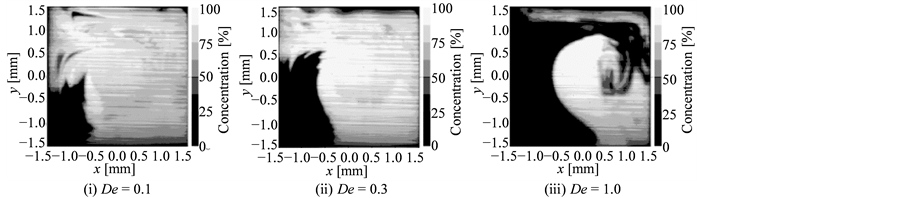 (c)
(c)
Figure 5. Concentration distribution of LIF at condition I. (a) Tr = 0; (b) Tr = 3; (c) Tr = −3.
 (a)
(a)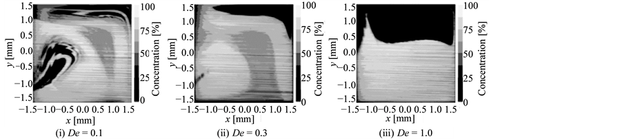 (b)
(b) (c)
(c)
Figure 6. Concentration distribution of LIF at condition II. (a) Tr = 0; (b) Tr = 3; (c) Tr = −3.

Figure 7. Concentration distribution of OpenFOAM at condition I. (a) Tr = 0; (b) Tr = 3; (c) Tr = −3.

Figure 8. Concentration distribution of OpenFOAM at condition II. (a) Tr = 0; (b) Tr = 3; (c) Tr = −3.
In Figure 7, the results at condition I are compared with the experimental results (Figure 5). For Tr = 0 (Figure 7(a)), the region with intermediate concentration (between 0 and 1) does not develop, although the boundary line between 100% and 0% regions is deformed due to the increase of the centrifugal force as De increases. Therefore, it is concluded that mixing is not promoted for this case. For Tr = 3 (Figure 7(b)), mixing is highly promoted at De = 0.1 and 0.3 of condition I and II as found from the enlargement of the intermediate region of concentration in the same manner as the experimental results. When De is increased up to 1.0, however, mixing is not effective as shown by the sharp separation of 100% and 0% regions, although the boundary is deformed similarly as the case for Tr = 0, which shows similar results to the experiment. For Tr = −3 (Figure 7(c)), the spatial structure of the mixing process is considerably different from those for Tr = 3, although occurrence or no occurrence of mixing is the same when De is changed. In the distribution of concentration, the results of numerical simulations closely agree with the experimental results. Then the result at condition II is compared with the experimental results (Figure 6) in Figure 8. We see that the tendency of the promotion of mixing is similar to condition I when Tr and De change as seen in the experimental results.
Therefore it is concluded that the numerical simulations are validated since the results of the numerical simulations reproduce the experimental results very well. Thus, the discussion on the physical mechanism of mixing will be conducted using the numerical simulation results.
4.3. Mixing Rate
Using the results of the numerical simulations, the mixing rate in the cross section at 180˚ is calculated. In order to quantitatively assess the effect of mixing, the mixture rate  [10] defined in Equation (5) is used
 . (5)
. (5)
In this equation  is the ratio of the fluid
  within the
  th small region, where the region of cross section is divided into
  small regions, and
  is as given by
 , (6)
, (6)
When the two fluids are completely mixed,  , and
, and  when no mixture occurs.
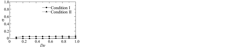
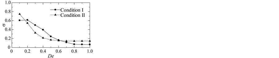
The mixing rate  at the two conditions is plotted as De changes for three cases for Tr in Figure 9. When Tr = 0, a slight increase of
  is observed as De increases. This is because the centrifugal force affects the interface deformation between the two fluids. It is notable that mixing is more promoted at condition I than condition II. However, the mixing rate is very small, and no effective mixing occurs.
For Tr = 3 and −3, the mixing rate is much greater than the case for Tr = 0, where no rotation is applied. On the other hand, it is interesting that the effect of the change of inflow condition of the concentration distribution is different for Tr > 0 or <0. Here we focus the secondary and axial flow velocities in the channel cross section.
For Tr = 3 as shown in Figure 9(b), the mixing rate  increases as De becomes smaller. This is mainly due to the effect of reversal flow, as shown in Figure 10(a), which exists from the channel center to the outer bottom region. In the region where De < 0.2, the reason of an inverted mixing rate is presumably caused by the effect of complex secondary flow shown in Figure 11(a), as well as the effect of reverse flow, in relation to the inflow conditions.
For Tr = −3 as shown in Figure 9(c), the mixing rate  increases as De becomes smaller, as the case for Tr = 3. This is due to the fact that mixing is promoted by the strong reverse flow as seen at the top side of the pictures in Figure 10(b). It is considered that the interface deformation is promoted particularly under the inflow condition II, which makes the mixing rate larger.
 (a) (b)
 (c)
(c)
Figure 9. Mixing rate in the cross section at 180˚. (a) Tr = 0; (b) Tr = 3; (c) Tr = −3.
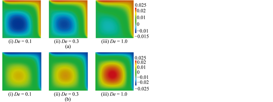
Figure 10. Axial flow patterns. (a) Tr = 3; (b) Tr = −3.
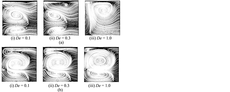
Figure 11. Secondary flow patterns. (a) Tr = 3; (b) Tr = −3.
5. Conclusions
In the present paper, we made the micromixer with a rotor and curved channel, which can mix very low Reynolds number flows efficiency, and obtained good agreement between experimental and numerical results:
When , mixing is highly promoted.
The highest mixing rate is  at the condition II for Tr = 3 and De = 0.1.
The inflow conditions at the entrance have large effect on the promotion of mixing, and the maximum promotion is achieved when the reverse flow due to rotation and secondary flow is combined.
Acknowledgements
The authors would like to express their cordial thanks to Naoyuki Yasuda and Koichiro Tabara for their help in the experiments.
References
- Stroock, A.D., Dertinger, S.K.W., Ajdari, A., Mezic, I., Stone, H.A. and Whitesides, G.M. (2002) Chaotic Mixer for Microchannels. Science, 295, 647-651. http://dx.doi.org/10.1126/science.1066238
- Kim, D.S., Lee, I.H., Kwon, T.H. and Cho, D.W. (2003) A Novel Chaotic Micromixer: Barrier Embedded Kenics Micromixer. Proceedings of 7th International Conference on Miniaturized Chemical and Biochemical Analysis Systems, Squaw Valley, 5-9 October 2003, 73-76.
- Sato, H., Ito, S., Tajima, K., Orimoto, N. and Shoji, S. (2005) PDMS Microchannels with Slanted Grooves Embedded in Three Walls to Realize Efficient Spiral Flow. Sensors and Actuators A: Physical, 119, 365-371. http://dx.doi.org/10.1016/j.sna.2004.08.033
- Niu, X.Z. and Lee, Y.-K. (2003) Efficient Spatial-Temporal Chaotic Mixing in Microchannels. Journal of Micromechanics and Microengineering, 13, 454-462. http://dx.doi.org/10.1088/0960-1317/13/3/316
- Tabeling, P., Chabert, M., Dodge, A., Jullien, C. and Okkels, F. (2004) Chaotic Mixing in Cross-Channel Micromixers. Philosophical Transactions of the Royal Society A, 362, 987-1000. http://dx.doi.org/10.1098/rsta.2003.1358
- Hayamizu, Y., Yanase, S., Morita, S., Ohtsuka, S., Gonda, T., Nishida, K. and Yamamoto, K. (2012) A Micromixer Using the Chaos of Secondary Flow: Rotation Effect of Channel on the Chaos of Secondary Flow. Open Journal of Fluid Dynamics, 2, 195-201. http://dx.doi.org/10.4236/ojfd.2012.24A021
- Yamamoto, K., Wu, X.Y., Nozaki, K. and Hayamizu, Y. (2006) Visualization of Taylor-Dean Flow in a Curved Duct of Square Cross-Section. Fluid Dynamics Research, 38, 1-18. http://dx.doi.org/10.1016/j.fluiddyn.2005.09.002
- The Japan Society of Mechanical Engineers (1971) JSME Data Book: Hydraulic Losses in Pipes and Ducts. The Japan Society of Mechanical Engineers, Tokyo, 68-72.
- OpenFOAM Official Site. http://www.openfoam.com/
- Funakoshi, M. (2008) Chaotic Mixing and Mixing Efficiency in a Short Time. Fluid Dynamics Research, 40, 1-33. http://dx.doi.org/10.1016/j.fluiddyn.2007.04.004