Paper Menu >>
Journal Menu >>
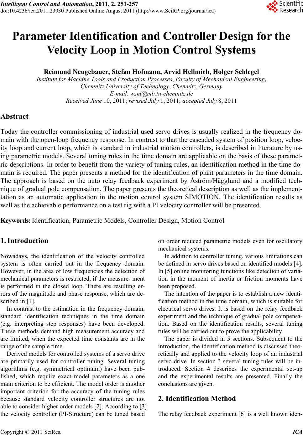 Intelligent Control and Automation, 2011, 2, 251-257 doi:10.4236/ica.2011.23030 Published Online August 2011 (http://www.SciRP.org/journal/ica) Copyright © 2011 SciRes. ICA Parameter Identification and Controller Design for the Velocity Loop in Motion Con tro l Systems Reimund Neugebauer, Stefan Hofmann, Arvid Hellmich, Holger Schlegel Institute for Machine Tools and Production Processes, Faculty of Mechanical Engineering, Chemnitz University of Technology, Chemnitz, Germany E-mail: wzm@mb.tu-chemnitz.de Received June 10, 2011; revised July 1, 2011; accepted July 8, 2011 Abstract Today the controller commissioning of industrial used servo drives is usually realized in the frequency do- main with the open-loop frequency response. In contrast to that the cascaded system of position loop, veloc- ity loop and current loop, which is standard in industrial motion controllers, is described in literature by us- ing parametric models. Several tuning rules in the time domain are applicable on the basis of these paramet- ric descriptions. In order to benefit from the variety of tuning rules, an identification method in the time do- main is required. The paper presents a method for the identification of plant parameters in the time domain. The approach is based on the auto relay feedback experiment by Åström/Hägglund and a modified tech- nique of gradual pole compensation. The paper presents the theoretical description as well as the implement- tation as an automatic application in the motion control system SIMOTION. The identification results as well as the achievable performance on a test rig with a PI velocity controller will be presented. Keywords: Identification, Parametric Models, Controller Design, Motion Control 1. Introduction Nowadays, the identification of the velocity controlled system is often carried out in the frequency domain. However, in the area of low frequencies the detection of mechanical parameters is restricted, if the measure- ment is performed in the closed loop. There are resulting er- rors of the magnitude and phase response, which are de- scribed in [1]. In contrast to the estimation in the frequency domain, standard identification techniques in the time domain (e.g. interpreting step responses) have been developed. These methods demand high measurement accuracy and are limited, when the expected time constants are in the range of the sample time. Derived models for controlled systems of a servo drive are primarily used for controller tuning. Several tuning algorithms (e.g. symmetrical optimum) have been pub- lished, which require exact model parameters as a one main criterion to be efficient. The model order is another important criterion for the accuracy of the tuning rules because standard velocity controller structures are not able to consider higher order models [2]. According to [3] the velocity controller (PI-Structure) can be tuned based on order reduced parametric models even for oscillatory mechanical systems. In addition to controller tuning, various limitations can be defined in servo drives based on identified models [4]. In [5] online monitoring functions like detection of varia- tion in the moment of inertia or friction moments have been proposed. The intention of the paper is to establish a new identi- fication method in the time domain, which is suitable for electrical servo drives. It is based on the relay feedback experiment and the technique of gradual pole compensa- tion. Based on the identification results, several tuning rules will be carried out to prove the applicability. The paper is divided in 5 sections. Subsequent to the introduction, the identification method is discussed theo- retically and applied to the velocity loop of an industrial servo drive. In section 3 several tuning rules will be in- troduced. Section 4 describes the experimental set-up and the experimental results are presented. Finally the conclusions are given. 2. Identification Method The relay feedback experiment [6] is a well known iden-  R. NEUGEBAUER ET AL. 252 tification approach, which is generally applied to identify a process Gs(s) on its limit of stability. For this purpose, the controller Gr(s) is replaced by a relay controller ac- cording to Figure 1. The original method provides a nonparametric model with the characteristics ultimate gain (ku) and ul- timate frequency (ωu). In contrast to that, the relay feed- back experiment is exclusively used as an excitation in the presented approach. The controlled variable x ap- pears as input for a compensator Gc(s). The aim is to adjust the compensator to the plant parameter by using the method of gradually compensation of the dominant pole [7]. This approach combines the advan- tages of the relay feedback experiment with those of the parametric model identification (Figure 1). For the example of a first order transfer function with dead time (FOPDT) a compensator (Gc) as shown in [8] is chosen. *1 1 d sT sc k Gse Gs Ts s Ts (1) Applying this, the forward path of the control loop becomes: *1 1 c d c yxs c sT Xs Gs GsGs Ys Ts ke sTs (2) Finally, this equation is expanded in terms of two components: * 1 1 d d sT c sT Xs keYs s TT ke Ys Ts (3) In the case of T* = T the term reduces to an integral plus dead time (IPDT) system: 1 d sT c X ske Ys s (4) As mentioned above, Y(s) is a relay output signal. With this input sequence, Equation (4) describes an ideal ramp function x(t). To adjust T*, Equation (3) needs to be evaluated to satisfy Equation (5): Figure 1. Identification with gradual pole compensation. * * 10 lim 1 d sT TT TT ke Ts s (5) To determine the compensator time constant T*, an adjustment criterion is of primary importance. Because of the expected small lag and dead times for electrical servo drives not all adjustment strategies are suitable. Consequently the oscillation magnitude of xc(t) is com- pared with the expected magnitude of the ramp function xi(t) (Figure 2) and T* is adjusted according to the mag- nitude ratio in Equation (6). ** 1 ˆ ˆ i nn c x TT x (6) For the evaluation, only the extreme values of xc(t) have to be determined, which entails a high toleration of measurement uncertainty even for lag times which are smaller than the sample time of the motion controller. The dead time of the system (Td) can be determined by the time behaviour of xc(t) and the relay output y(t) [9]. 2.1. Velocity Control Loop The velocity controller (GVC) is typically implemented as PI controller. The subordinated system consists of the closed current loop (GCuL) and a mechanical system (Gmech) which is mainly characterized by the total mo- ment of inertia J and an oscillatory system. The resulting structure with an additional nonlinear friction moment (Mfric) is displayed in Figure 3. 2.2. Identification of the Velocity Controlled System The derivation of a parametric model of the velocity controlled system consists of three steps. In the first step, the closed current loop is described by using the FOPDT identification approach, introduced in Section 2. In a second step, it is shown, how the proposed adjustment strategy can be applied to a first order plus integral plus Figure 2. Proposed criterion for compensator adjustment. Figure 3. Structure of the velocity control loop. Copyright © 2011 SciRes. ICA 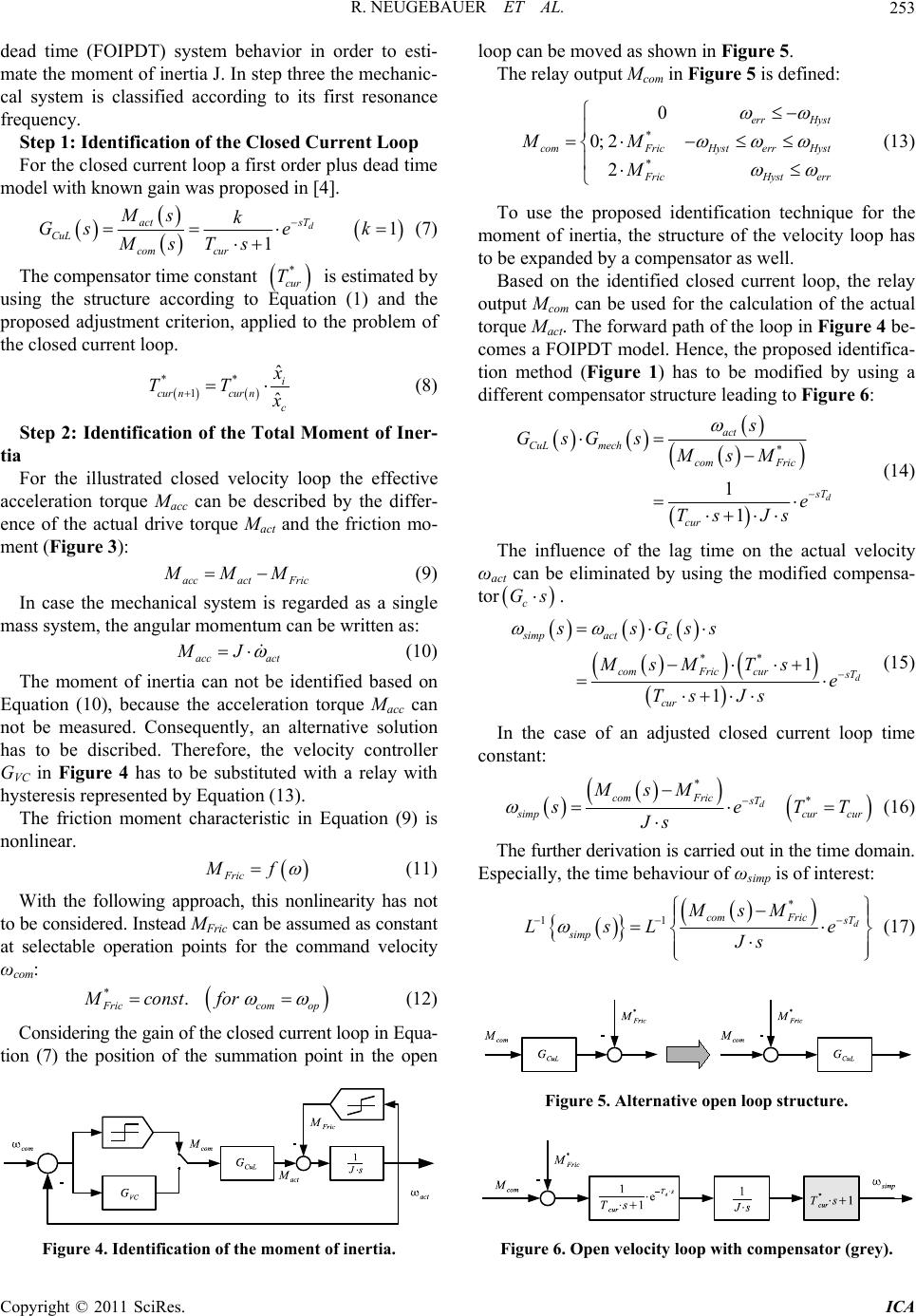 R. NEUGEBAUER ET AL.253 dead time (FOIPDT) system behavior in order to esti- mate the moment of inertia J. In step three the mechanic- cal system is classified according to its first resonance frequency. Step 1: Identification of the Closed Current Loop For the closed current loop a first order plus dead time model with known gain was proposed in [4]. 1 1 d sT act CuL com cur Ms k Gse k MsTs (7) The compensator time constant is estimated by using the structure according to Equation (1) and the proposed adjustment criterion, applied to the problem of the closed current loop. * cur T ** 1 ˆ ˆ i cur ncur n c x TT x (8) Step 2: Identification of the Total Moment of Iner- tia For the illustrated closed velocity loop the effective acceleration torque M acc can be described by the differ- ence of the actual drive torque Mact and the friction mo- ment (Figure 3): accact Fric MMM (9) In case the mechanical system is regarded as a single mass system, the angular momentum can be written as: acc act MJ (10) The moment of inertia can not be identified based on Equation (10), because the acceleration torque Macc can not be measured. Consequently, an alternative solution has to be discribed. Therefore, the velocity controller GVC in Figure 4 has to be substituted with a relay with hysteresis represented by Equation (13). The friction moment characteristic in Equation (9) is nonlinear. Fric Mf (11) With the following approach, this nonlinearity has not to be considered. Instead MFric can be assumed as constant at selectable operation points for the command velocity ωcom: *. F riccom op Mconstfor (12) Considering the gain of the closed current loop in Equa- tion (7) the position of the summation point in the open Figure 4. Identification of the moment of inertia. loop can be moved as shown in Figure 5. The relay output Mcom in Figure 5 is defined: * * 0 0; 2 2 err Hyst comFricHyst errHyst F ricHysterr MM M (13) To use the proposed identification technique for the moment of inertia, the structure of the velocity loop has to be expanded by a compensator as well. Based on the identified closed current loop, the relay output Mcom can be used for the calculation of the actual torque Mact. The forward path of the loop in Figure 4 be- comes a FOIPDT model. Hence, the proposed identifica- tion method (Figure 1) has to be modified by using a different compensator structure leading to Figure 6: * 1 1 d act CuL mech com Fric s T cur s GsG s MsM e Ts Js (14) The influence of the lag time on the actual velocity ωact can be eliminated by using the modified compensa- tor c Gs . ** 1 1 d simpact c comFric cur s T cur ssGss MsMTs e Ts Js (15) In the case of an adjusted closed current loop time constant: * * d comFric sT s impcur cur MsM seTT J s (16) The further derivation is carried out in the time domain. Especially, the time behaviour of ωsimp is of interest: * 11 d comFric sT simp MsM LsL e Js (17) Figure 5. Alternative open loop structure. Figure 6. Open velocity loop with compensator (grey). Copyright © 2011 SciRes. ICA 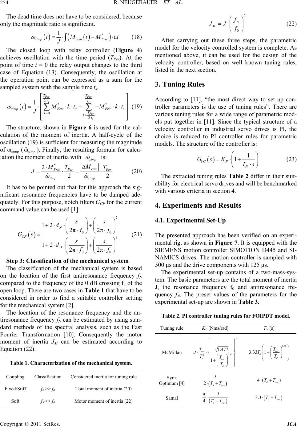 R. NEUGEBAUER ET AL. 254 The dead time does not have to be considered, because only the magnitude ratio is significant. * 1d simpcom Fric tMtMt J (18) The closed loop with relay controller (Figure 4) achieves oscillation with the time period (TPer). At the point of time t = 0 the relay output changes to the third case of Equation (13). Consequently, the oscillation at the operation point can be expressed as a sum for the sampled system with the sample time ts. 2** 0 2 1 Per Per ss Per s TT tt s impFric sFrics T kkt tMktMk J t (19) The structure, shown in Figure 6 is used for the cal- culation of the moment of inertia. A half-cycle of the oscillation (19) is sufficient for measuring the magnitude of ωsimp (simp ). Finally, the resulting formula for calcu- lation the moment of inertia with ˆ ω ˆ s imp is: * 2 ˆˆ 22 com F ric PerPer simp simp M M T J T (20) It has to be pointed out that for this approach the sig- nificant resonance frequencies have to be damped ade- quately. For this purpose, notch filters GCF for the current command value can be used [1]: 2 0 2 00 12 2π2π 12 2π2π N CF D ss dff Gs ss dff 0 (21) Step 3: Classification of the mechanical system The classification of the mechanical system is based on the location of the first antiresonance frequency fN compared to the frequency of the 0 dB crossing fd of the open loop. There are two cases in Table 1 that have to be considered in order to find a suitable controller setting for the mechanical system [2]. The location of the resonance frequency and the an- tiresonance frequency fN can be estimated by using stan- dard methods of the spectral analysis, such as the Fast Fourier Transformation [10]. Consequently the motor moment of inertia JM can be estimated according to Equation (22). Table 1. Characterization of the mechanical system. Coupling Classification Considered inertia for tuning rule Fixed/Stiff fN >> fd Total moment of inertia (20) Soft fN << fd Motor moment of inertia (22) 2 0 N M f JJ f (22) After carrying out these three steps, the parametric model for the velocity controlled system is complete. As mentioned above, it can be used for the design of the velocity controller, based on well known tuning rules, listed in the next section. 3. Tuning Rules According to [11], “the most direct way to set up con- troller parameters is the use of tuning rules”. There are various tuning rules for a wide range of parametric mod- els put together in [11]. Since the typical structure of a velocity controller in industrial servo drives is PI, the choice is reduced to PI controller rules for parametric models. The structure of the controller is: 1 1 VC P N GsKTs (23) The extracted tuning rules Table 2 differ in their suit- ability for electrical servo drives and will be benchmarked with various criteria in section 4. 4. Experiments and Results 4.1. Experimental Set-Up The presented approach has been verified on an experi- mental rig, as shown in Figure 7. It is equipped with the SIEMENS motion controller SIMOTION D445 and SI- NAMICS drives. The motion controller is sampled with 500 μs and the drive components with 125 μs. The experimental set-up contains of a two-mass-sys- tem. The basic parameters are the total moment of inertia J, the resonance frequency f0 and antiresonance fre- quency fN. The preset values of the parameters for the experimental set-up are shown in Table 3. Table 2. PI controller tuning rules for FOIPDT model. Tuning rule KP [Nms/rad] TN [s] McMillan 2 0.65 2 1.477 1 cur dcur d T JTT T 0.65 3.33 1cur d d T TT Sym. Optimum [4] 2dcur J TT 4dcur TT Samal π 4dcur J TT 3.3 dcur TT Copyright © 2011 SciRes. ICA  R. NEUGEBAUER ET AL.255 Figure 7. Experiment set-up with motion controller. Table 3. Parameters of the experimental set-up. Configuration J [kgm²] f0 [Hz] fN [Hz] Two-mass-system (Stiff coupling) 6 1355 10 422 333 4.2. Identification Results The closed current loop (7) under relay feedback and the identified model are shown in the following time plot. The identified model has been calculated in the sample time of the motion controller. Even for a lag time which is smaller than the sample time, the reaction curves of the real values and the modelled values are nearly identical Figure 8. Hence, the performance of the chosen adjustment strategy is proven. According to Equation (13), the hysteresis of the relay is a free selectable parameter. Therefore, a compromise between the magnitude of the relay oscillation and the linearization error for the friction moment (12) has to be found. The moment of inertia for the mechanical system at different operation points is plotted with a variable hysteresis in Figure 9. The graph demonstrates that the value of the moment of inertia for the mechanical system can be identified with sufficient accuracy. A variance of less than 4% can be achieved for a hysteresis to operation point ratio >0.1. Comparing the achieved moments of inertia to other in- vestigations [12,13], the experiments have shown an im- provement of the accuracy. Simultaneously, a small value of the velocity (operation point) is sufficient. Hen- ce, the stress to the mechanical system is smaller. Conse- Figure 8. Time behavior of closed current loop. Figure 9. Results for the total moment of inertia. quently the FOIPDT model (14) can be written with the identified parameters. 4.3. Controller Design Using the identified parametric model from Table 4 and the tuning rules for PI controller from Table 2, the achievable phase margin and gain margin can be calcu- lated. The typical phase margin for set point response is a range of 70° - 40° and for disturbance response a range of 50° - 20° [4]. As it is recognizable in Table 5, all listed tuning rules can be classified as sufficient for a good disturbance response. 4.4. Achievable Results The behavior of these tuning rules on disturbance steps is shown in Figure 10. In addition, the internal tuning rule of the drive system is listed as “automatic”. The introduced tuning rules show a better disturbance response, compared to the automatic tuning of the drive system. As expected from the open loop stability calcu- lation Table 5, McMillan and Samal have the smallest settling times. Table 4. Identified parameters for controller design. Model J [kgm²] Td [s] Tcur [s] 1 d sT cur e J Ts s 6 1340 10 3 0.25 10 3 0.4 10 Table 5. Estimated open loop characteristics. Tuning rulefd [Hz] Gain margin [dB] Phase margin [°] McMillan 238 5.91 19.2 Sym. Optimum 129 13.3 35 Samal 188 8.76 25.9 Copyright © 2011 SciRes. ICA 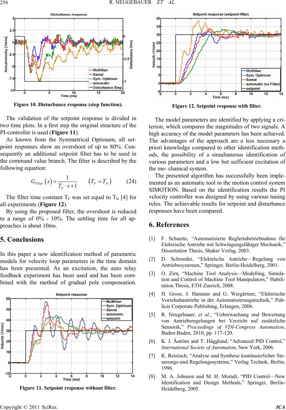 R. NEUGEBAUER ET AL. 256 Figure 10. Disturbance re sponse (ste p function). The validation of the setpoint response is divided in two time plots. In a first step the original structure of the PI-controller is used (Figure 11). As known from the Symmetrical Optimum, all set- point responses show an overshoot of up to 80%. Con- sequently an additional setpoint filter has to be used in the command value branch. The filter is described by the following equation: 1 1 F ilterF N F Gs TT Ts (24) The filter time constant TF was set equal to TN [4] for all experiments (Figure 12). By using the proposed filter, the overshoot is reduced to a range of 0% - 10%. The settling time for all ap- proaches is about 10ms. 5. Conclusions In this paper a new identification method of parametric models for velocity loop parameters in the time domain has been presented. As an excitation, the auto relay feedback experiment has been used and has been com- bined with the method of gradual pole compensation. Figure 11. Setpoint respon se without filter. Figure 12. Setpoint response with filter. The model parameters are identified by applying a cri- terion, which compares the magnitudes of two signals. A high accuracy of the model parameters has been achieved. The advantages of the approach are a less necessary a priori knowledge compared to other identification meth- ods, the possibility of a simultaneous identification of various parameters and a low but sufficient excitation of the me- chanical system. The presented algorithm has successfully been imple- mented as an automatic tool in the motion control system SIMOTION. Based on the identification results the PI velocity controller was designed by using various tuning rules. The achievable results for setpoint and disturbance responses have been compared. 6. References [1] F. Schuette, “Automatisierte Reglerinbetriebnahme für Elektrische Antriebe mit Schwingungsfähiger Mechanik,” Dissertation Thesis, Shaker Verlag, 2003. [2] D. Schroeder, “Elektrische Antriebe—Regelung von Antriebssystemen,” Springer, Berlin-Heidelberg, 2001. [3] O. Zirn, “Machine Tool Analysis—Modelling, Simula- tion and Control of Machine Tool Manipulators,” Habili- tation Thesis, ETH Zuerich, 2008. [4] H. Gross, J. Hamann and G. Wiegärtner, “Elektrische Vorschubantriebe in der Automatisierungstechnik,” Pub- licis Corporate Publishing, Erlangen, 2006. [5] R. Neugebauer, et al., “Ueberwachung und Bewertung von Antriebsregelungen bei Verzicht auf zusätzliche Sensorik,” Proceedings of VDI-Congress Automation, Baden-Baden, 2010, pp. 117-120. [6] K. J. Åström and T. Hägglund, “Advanced PID Control,” International Society of Automation, New York, 2006. [7] K. Reinisch, “Analyse und Synthese kontinuierlicher Ste- uerungs-und Regelungssysteme,” Verlag Technik, Berlin, 1996. [8] M. A. Johnson and M. H. Moradi, “PID Control—New Identification and Design Methods,” Springer, Berlin- Heidelberg, 2005. Copyright © 2011 SciRes. ICA 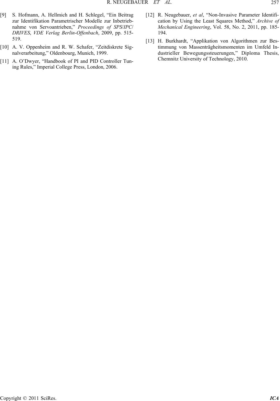 R. NEUGEBAUER ET AL. Copyright © 2011 SciRes. ICA 257 [9] S. Hofmann, A. Hellmich and H. Schlegel, “Ein Beitrag zur Identifikation Parametrischer Modelle zur Inbetrieb- nahme von Servoantrieben,” Proceedings of SPS/IPC/ DRIVES, VDE Verlag Berlin-Offenbach, 2009, pp. 515- 519. [10] A. V. Oppenheim and R. W. Schafer, “Zeitdiskrete Sig- nalverarbeitung,” Oldenbourg, Munich, 1999. [11] A. O’Dwyer, “Handbook of PI and PID Controller Tun- ing Rules,” Imperial College Press, London, 2006. [12] R. Neugebauer, et al, “Non-Invasive Parameter Identifi- cation by Using the Least Squares Method,” Archive of Mechanical Engineering, Vol. 58, No. 2, 2011, pp. 185- 194. [13] H. Burkhardt, “Applikation von Algorithmen zur Bes- timmung von Massenträgheitsmomenten im Umfeld In- dustrieller Bewegungssteuerungen,” Diploma Thesis, Chemnitz University of Technology, 2010. |