Received 12 February 2016; accepted 21 March 2016; published 24 March 2016

ABSTRACT

This paper provides a proof of the well-known relationship between the pure delay and the natural period of oscillation in industrial systems.

Keywords:

Pure Delay, Period of Oscillation, First Order Systems, PID Control

1. Introduction and Hypothesis

The approximate relationship

(1)

between the pure delay T_u and the natural period of oscillation P_n in industrial systems is well known to control engineers.

This relationship is in the core of the PID [1] tuning rules designed by Ziegler and Nichols [2] . If the values of integral times T_i in the methods of closed loop and open loop are equated, it comes down to

(2)

Solving the right side equation for P_n, (1) is reached. So, this relationship is widely used in practice to verify the identification of pure delay, which is not always easy to measure, and then calculate the parameters of PID controllers. However, it is remarkable that it has not received sufficient attention in academia.

This paper presents a demonstration of this relationship based on the behavior of first order systems with pure delay, using basic tools of linear control as root locus and polynomial algebra.

2. Proof

Since P_n = 1/f_n, where f_n is de oscillation frequency, and the angular natural frequency is w_n = 2πf_n, the natural period can be written as P_n = 2π/w_n. Substituting this value in Equation (1), this becomes to

(3)

Solving this equation for w_n, an equivalent expression to Equation (1) is derived:

(4)

Now, the most of industrial processes can be modeled by first order systems with pure delay, which have the Laplace transfer function [3]

(5)

In this equation, K_e is the static gain and T_g the process time constant.

For the purpose of finding the characteristic equation of the system, the pure delay can be represented by the second order Padé approximation [4] :

(6)

Then, G(s) is approximated as

(7)

The characteristic equation of the system is obtained by adding numerator and denominator of Equation (7):

(8)

It is necessary to find the value of the static gain K_e where a pair of complex conjugate roots reaches the imaginary axis and the system becomes oscillatory with a natural frequency w_n.

For readability, each coefficient of Equation (8) is identified as C_i. It is then

(9)

To be sure that the roots of this equation are in the left half-plane, a first requirement is that all coefficients are positive. In other words, a limit gain K_e can be found when any of these coefficients are set to zero. The only one who is able to accomplish this is C₂:

(10)

Solving for K_e, a first value K_el1 of a limit gain is then obtained:

(11)

Now it must be determined if other values of K_e can produce imaginary roots in Equation (8). The Routh arrangement [5] of the characteristic equation is constructed for this purpose:

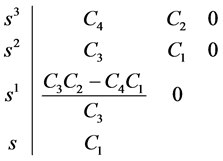(12)

As stated in Rooth-Hurwitz criterion [6] , the system poles are in the left half plane if there are no sign changes in the first column of the array, and the point where a root is located over the imaginary axis can be found by canceling any of its elements. The only element that is able to be null is the one for s¹. Therefore, and considering that is always positive, the condition can be written as.

This corresponds to

(13)

Solving this equation for K_e, there are two new values K_el2 wherein the real part of the roots is canceled:

(14)

It is easy to show that K_el2a meets the condition of being positive and is also lower than the value of K_el1 given by Equation (11). Therefore K_el2a shall be the gain value that defines the point of oscillation of the system.

Then, to find the oscillation frequency of the system, K_el2a can be replaced into the characteristic Equation (8) and solving it for the values of s, which should be imaginary. However, this way the algebra becomes somewhat tangled. Therefore a property of polynomials is used, which states that secondary equations of the Routh arrangement (12) have roots that satisfy the characteristic equation. In particular, the auxiliary equation corresponding to s² does not have odd powers, so it has symmetric roots with imaginary values:

(15)

The roots of this equation are

(16)

So the natural angular frequency w_n is

(17)

Now, in this equation the gain K_e must be replaced by the value K_el2a that brings the system to the oscillation, obtained in Equation (14). This leads to

(18)

In most industrial systems the pure delay T_u is significantly lower than the time constant T_g, i.e.. So T_u can be omitted when appears beside T_g in Equation (18). With this consideration, w_n is expressed approximately as

(19)

This value is almost coincident with the stated by Equation (4), which finally proof the hypothesis in Equation (1).

Cite this paper

DanielChuk,Gustavo RodriguezMedina, (2016) On the Relationship between the Pure Delay and the Natural Period of Oscillation. Applied Mathematics,07,504-507. doi: 10.4236/am.2016.76046

References

- 1. O’Dwyer, A. (2006) Handbook of PI and PID Controller Tuning Rules. 2nd Edition, Imperial College Press, 78.
- 2. Ziegler, J.G. and Nichols, N.B. (1942) Optimum Settings for Automatic Controllers. Transactions of the ASME, 64,759-768.
- 3. Ogata, K. (2003) Ingeniería de control moderna. Pearson Educación, S.A., Madrid.
- 4. Cai, J., King, J.B., Merrick, B.M. and Brazil, T.J. (2013) Padé-Approximation-Based Behavioral Modeling. IEEE Transactions on Microwave Theory & Techniques, 61, 4418-4427.
http://dx.doi.org/10.1109/TMTT.2013.2287677 - 5. Kavitha, P. and Ramakalyan, A. (2014) Simple and Straight Proofs of Stability Criteria for Finite-Dimensional Linear Time Invariant Systems. Transactions of the Institute of Measurement & Control, 36, 523-528.
http://dx.doi.org/10.1177/0142331213510548 - 6. Choghadi, M.A. and Talebi, H.A. (2013) The Routh-Hurwitz Stability Criterion, Revisited: The Case of Multiple Poles on Imaginary Axis. IEEE Transactions on Automatic Control, 58, 1866-1869.
http://dx.doi.org/10.1109/TAC.2013.2242591