World Journal of Engineering and Technology
Vol.04 No.02(2016), Article ID:66323,10 pages
10.4236/wjet.2016.42017
RapidSCAT Sigma-0 and Tb Measurements Validation
Patrick Fiati
Department of Electrical, Electronic Engineering, Kwame Nkrumah University of Science and Technology, Kumasi, Ghana
![]()
Copyright © 2016 by author and Scientific Research Publishing Inc.
This work is licensed under the Creative Commons Attribution International License (CC BY).
http://creativecommons.org/licenses/by/4.0/


Received 20 January 2016; accepted 7 May 2016; published 10 May 2016
ABSTRACT
Scatterometer Radar Backscatter Calibration since the first SeaSat-A Satellite Scatterometer (Birer et al., 1982), the Amazon tropical rain forest has been recognized as a spatially large extent, homogeneous radar calibration target. During the commissioning of NSCAT (1996) and later QuikSCAT (1999), CFRSL worked with the JPL Scatterometer Cal/Val team to perform normalized radar cross section (Sigma-0) calibrations using the Amazon (see Zec et al., 1999-A and 1999-B) [1] . It is important to continue this activity using RapidSCAT to validate the Sigma-0 measurement provided in the L-1A data product, and moreover the time series of these backscatter observations can be used to establish an improved Ku-band Amazon calibration site for future on-orbit radar calibration [2] . Unfortunately, the Amazon radar backscatter (Sigma-0) exhibits a time of day dependence that is not well characterized, and for the sun-synchronous polar orbiting satellites (SeaSat-A, ADEOS-I and QuikSCAT), the observations occur at specific times of day, during the morning and night passes. But now with the low-earth-orbit of the ISS, there will be an orderly orbit precession, which allows the region to be uniformly sampled over the 24-hour period [3] . Also, since the RapidSCAT employs a conical scanning geometry, we can examine the isotropic nature of Amazon backscatter established by Zec’s (1998-A) analysis of NSCAT and later (1999-B) of QuikSCAT observations [4] . Thus, observations, collected over the RapidSCAT two-year mission will sample the Amazon with high spatial/temporal resolution, as a function of time of day, and over seasons. We propose to analyze these data to develop a high spatial resolution Sigma-0 Amazon map that can be used by future satellite radar missions.
Keywords:
RapidSCAT, QuikSCAT, Scatterometer, HIRAD, Sigma-0

1. Introduction
Scatterometer Radiometric Brightness Temperature previously under the QuikSCAT program, the LL developed a QRad brightness temperature (Tb) measurement capability included in the scatterometer L-1B data product. This Tb measurement was implemented using the QuikSCAT L-1A and L-1B data products during ground data processing at the JPL PODAAC [5] . The QRad Tb had been shown by Ahmed et al. (2005) to be capable of providing measurements of rain simultaneous with the scatterometer backscatter measurements. As such, it could provide a reliable rain flag (e.g., used in the MUDD rain flag) or independent measurements (Tbh & Tbv) for use in an active/passive OVW retrieval algorithm (Laupattarakasem et al. (2009) and Alsweiss et al. (2011)) [6] .
Previously, when SeaWinds flew on ADEOS-II, there was a significant degradation of the QRad Tb’s because of physical temperature changes in the QSCAT antenna and waveguides during the orbit day/night periods. CFRSL developed an empirical correction algorithm that was implemented by PODAAC; however the QRad Tb was adversely compromised as reported by Rastogi et al. (2005) [7] .
The Tb measurement capability on RapidSCAT will also suffer because of the ISS day/night periods, which occur every orbit. However, based upon the CFRSL Intersatellite Radiometric Calibration (XCAL) experience on the TRMM Microwave Imager, an effective procedure has been developed by Biswas (2010) to remove the time varying orbit Tb bias from the TMI radiometer. We propose to apply this method for RapidSCAT and to perform continuous XCAL with the Global Precipitation Mission Microwave Imager (GMI). These XCAL evaluations will validate the effectiveness of the RapidSCAT Tb algorithm for providing accurate ocean Tb’s [8] .
1.1. Objectives
This research entails finding a bug in current HiRAD processing software and fixing it.
・ Level_0a: Dump of raw data into MATLAB mat files: Moments 1 - 4 + cross-correlations between phase and quadrature signal components. Most useful are second moments files containing time reference and telemetry information.
・ Level_0b: Data organized in channels, time stamps and type (warm/cold load, isolator, etc.).
・ Level_0c: Same as Level_0b, but interpolated to the same time grid since various Level_0b data are in different time slices.
Level_0c is the input to processing. Many Tb images show artificial stripes and goal is to detect the source of this error and remove it.
1.2. Active/Passive Hurricane OVW Retrievals
Historically, scatterometer OVW retrievals in hurricanes have badly under estimated ocean surface wind speeds > 30 m/s (hurricane CAT-1). The two main reasons are: Sigma-0 saturation at high wind speeds and the atmospheric attenuation associated with heavy tropical rain bands.
Concerning the first, airborne scatterometer measurements in hurricanes by Esteban-Fernandez, et al. (2006) indicate that the Sigma-0 geophysical model function (GMF) increase until wind speeds reach 50 m/s (V-pol) or 70 m/s (H-pol); however these high wind speeds occur in limited spatial extent < 10 km. The smaller antenna beam footprints for RapidSCAT (compared to QuikSCAT) will allow better beam slices that should yield better OVW retrievals.
Concerning the rain attenuation issue, research conducted with QuikSCAT by CFRSL by Laupattarakasem et al. (2009) and Alsweiss et al. (2011) has shown promise that combined active/passive OVW retrievals algori- thms can significantly improve high wind speed retrievals. Further, with the lower altitude of the ISS and the resulting smaller SCAT antenna footprints will result in improved OVW retrieval performance.
We propose to use RapidSCAT hurricane observations with near coincident aircraft under-flights to tune our active/passive OVW retrieval algorithm. Further, after developing this algorithm, it will be applied to SeaWinds on ADEOS-II and QuikSCAT measurements in hurricanes. By cross comparison of these hurricane retrievals with RapidSCAT, we will investigate the effects of spatial scaling on the active/passive OVW retrieval algo- rithm for future scatterometers [9] .
2. Methodology
Forward models are presented which relate HIRAD’s raw radiometric self and cross-correlations to the antenna temperature  and visibility (V) incident on the antenna and to the brightness temperatures of the internal calibration reference sources. These models are inverted to solve for
  and V using measurements made while viewing the antenna and the calibration sources.
2.1. Self Correlation Forward Model
The basic signal flow through the radiometer for self-correlation measurements made by individual HIRAD receivers is shown in Figure 1.
In Figure 1, TA is the incident brightness temperature weighted by the antenna pattern of an individual HIRAD 16-element linear array antenna, L is the net transmissivity of the lossy radome and antenna, Tiso is the physical temperature of the isolator that is connected to the antenna (it is used as an estimate of the physical temperature of the radome and antenna),  is the effective antenna temperature after propagation through the radome and antenna (including self emission by the lossy elements), TW and TC are the brightness temperatures of the internal warm and cold calibration loads, TND is the increase in brightness temperature due to the noise diode (which includes the effects of losses due to power division, cable losses and the directional coupler), G is the receiver gain in units of Kelvins/counts, and CX is the raw 2nd moment counts when the system is in state X. Possible system states include: X = A (viewing the antenna), W (warm load), C (cold load), W + ND (warm load with noise diode on), and C + ND (cold load with noise diode on) [10] .
Note that hardware problems have been identified that affect the stability of the noise diode signal in some channels some of the time. For this reason, a version of the calibration is described here which does not use the noise diode measurements.
The forward model expression for CX while viewing the antenna is given by
 (1)
(1)
where ![]() is the portion of the receiver noise temperature that is common to the antenna and calibration views,
is the portion of the receiver noise temperature that is common to the antenna and calibration views, ![]() is the difference between the cal and non-cal receiver noise temperature,
is the difference between the cal and non-cal receiver noise temperature, ![]() is a possible digital offset, and
is a possible digital offset, and ![]() is given by
is given by
![]() (2)
(2)
The 2nd moment counts while viewing the calibration states are given by
![]() (3)
(3)
![]() (4)
(4)
2.2. Antenna Temperature Calibration Algorithm
The TA calibration algorithm is derived by appropriate manipulation of Equations (1)-(4). The gain is found from (3) and (4) as
![]() (5)
(5)
The antenna temperature is found from (1)-(3) as
![]() (6)
(6)
and
![]() (7)
(7)
Equations (5)-(7) constitute the zero’th visibility (V0) calibration algorithm [11] .
2.3. Cross Correlation Forward Model
The basic signal flow through the radiometer for cross-correlation measurements made by pairs of HIRAD receivers is shown in Figure 2.

Figure 1. Signal flow diagram for HIRAD self correlation measurements.
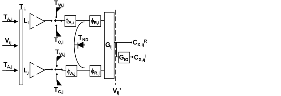
Figure 2. Signal flow diagram for HIRAD cross correlation measurements.
In Figure 2, incident  signals enter the ith and jth channels of HIRAD. The antenna transmissivity, L, and the warm and cold reference brightness temperatures,
  and
and , are in general different for each channel. The total phase transfer of the signal from the ith antenna to the correlator is

where  represents the portion of the signal path prior to the noise diode coupler and
  represents the portion that also affects the injected noise diode signal. A single noise diode is common to all ten HIRAD channels to provide a correlated signal, but its additive brightness temperature is in general different for each channel.
  is the cross-correlation gain for the ith and jth channels.
  and
and  represent the real and imaginary components of the raw cross-correlation counts when the system is in state X, and
  represents the gain imbalance between the two complex components.
In practice, the real and imaginary components of the cross-correlation counts are computed by multiplying and accumulating the proper in-phase and quadrature components of the signals from the two channels. If the in-phase and quadrature components of the signal from the ith channel are defined as  and
and , respectively, the cross-correlation counts are given by
 (8a)
(8a)
and
 (8b)
(8b)
The incident visibility sample corresponding to the baseline separation between the ith and jth antennas is defined as
 (9)
(9)
The incident visibility is attenuated by the lossy radome and antenna in a manner similar to the incident antenna temperature. However, because the visibility is formed by the product of the signals incident on each antenna, it will be attenuated by the geometric mean of the individual transmissivities. Therefore, the effective transmissivity of the lossy radome and antenna with respect to propagation by visibility  is given by
 (10)
(10)
The complex phase angle of the visibility will be rotated due to differences in phase transfer between the signals paths from the two antennas to the common correlator. The component of the difference in phase transfer that is common to both the antenna and noise diode signals can result from differences in the phase transfer functions of the two receivers, differences in the phase of the local oscillator signals arriving at each receivers down conversion mixer, and from differences in the lengths of the transmission lines from the receivers to the correlator. The component of the difference in phase transfer that occurs before the noise diode coupler (and is therefore not tracked by noise diode deflection measurements) can result from differences in the phase transfer functions of the two antennas and beam formers [12] .
If the difference in phase transfer between the two antenna signals is given by

then the measured visibility, V’, will be a rotated version of the actual visibility, V, described by
 (11a)
(11a)
and
 (11b)
(11b)
The rotated visibility, V’, is what is actually correlated. The forward model expressions for the real and imaginary parts of the raw correlation counts while viewing the antenna,  and
and , are given by
 (12a)
(12a)
and
 (12b)
(12b)
where  and
and  are residual offsets in the correlation counts, due at least in part to offsets between the analog and digital ground potentials at the digitization stage. These offsets should in practice be quite small and stable [13] .
The cross-correlation counts measured while viewing the warm and cold calibration sources are given by
 (13)
(13)
and
 (14)
(14)
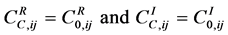
Equations (13) and (14) assume there is no correlated signal present in either the warm or cold load cali- bration states because the loads are different for each channel and so generate uncorrelated noise.
A common noise diode is split by an in-phase power divider and coupled into the receiver front end of each channel, as noted schematically in Figure 2. The maximum possible cross-correlation between the noise diode signals in the ith and jth channels is given by
 (15)
(15)
where  is the increase in brightness temperature due to the noise diode for the ith channel. This maximum is achieved if the two noise diode signals incident on the cross-correlator are in phase. Ideally, the noise diode signal should be injected in phase into each receiver (and cable lengths have been carefully matched to ensure this). However, differences in phase transfer between channels, similar to those experienced by the antenna signals noted above, will cause the complex correlation between the noise diode signals in each channel to also rotate. The rotation angle may differ from that of the antenna signals because they do not share identical propa- gation paths. If the complex phase rotation angle of the noise diode signal is
 , then the measured complex cross-correlation will be given by
 (16a)
(16a)
and
 (16b)
(16b)
where it is assumed that there is no intrinsic imaginary component of the cross-correlation prior to the differen- tial phase change [14] .
2.4. Visibility Gain Calibration
The visibility calibration algorithm is derived by appropriate manipulation of Equations (8)-(14). The cross- correlation offsets,  and
and , are determined directly from either the warm or cold load counts according to (13) and (14). The cross-correlation gain is found as the geometric mean of the appropriate pair of self-corre- lation gains. If Gi is the self-correlation gain for receiver i, given by (5), then
 (17)
(17)
The rotated visibility, V’, is found from Equation (12) as
 (18a)
(18a)
and
 (18b)
(18b)
2.5. Visibility Phase Calibration
The complex phase rotation angle of the noise diode correlation,  in Equation (16), is given by
 (19)
(19)
where the  function should take account of the possibility that the rotation angle will lie in the 3rd or 4th quadrant of the complex plane if the denominator in Equation (19) is negative.
Phase calibration of the visibility measured while viewing the antenna should ideally consist of counter- rotating the measured visibility, V’, by a complex angle  (see Equation (11)). However, variations in the difference between the portions of the ith and jth antenna signal path that lie outside the noise diode calibration loop (i.e. variations in
 ) are assumed to be negligible and phase calibration of the visibility only corrects for variations in
 . The phase calibration algorithm is given by
 (20a)
(20a)
and
 (20b)
(20b)
where  and
and  are given by Equation (18) and
  is given by Equation (19).
3. Analysis
HIRAD Visibility Calibration Algorithm.
The visibility function  resulting from this distribution is found from

The estimated brightness temperature of the image at  is given as
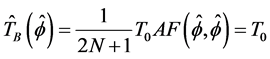

 (20)
(20)


4. Conclusions
This research entails developing empirical formulations or algorithms which will help in the visibility of the calibrations on the radiometer.
To help reduce the errors in the visibility, the equipment is injected with noise using the noise diode or noise generator.
From the formulations above, there is a link between visibility  and the noise error
  from the warm and cold temperature and Noise Diode Temperature (
 ).
).
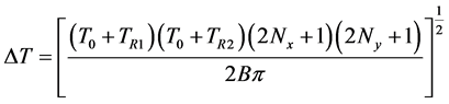
 depends on the available integration time, system bandwidth, receiver noise temperature, and the brightness temperature distribution.
 ’s are then translated into brightness temperature errors, or
 ’s, via the image reconstruction process in pixels.
 is the source of error.
Cite this paper
Patrick Fiati, (2016) RapidSCAT Sigma-0 and Tb Measurements Validation. World Journal of Engineering and Technology,04,183-192. doi: 10.4236/wjet.2016.42017
References
- 1. Newton, R.W. and Rouse Jr., J.W. (1980) Microwave Radiometer Measurements of Soil Moisture Content. IEEE Transactions on Antennas and Propagation, AP-28, 680-686.
- 2. Blume, H.-J.C., Kendall, B.M. and Fedors, J.C. (1978) Measurement of Ocean Temperature and Salinity via Microwave Radiometry. Boundary-Layer Meteorology, 134, 295-308.
http://dx.doi.org/10.1007/BF00913879 - 3. Pawsey, J.L. and Bracewell, R.N. (1955) Radio Astronomy. Oxford University Press, Oxford.
- 4. Kraus, J.D. (1966) Radio Astronomy. McGraw-Hill, New York.
- 5. Verschuur, G.L. and Kellermann, K.I. (1974) Galactic and Extra-Galactic Radio Astronomy. Springer-Verlag, Berlin.
- 6. Le Vine, D.M., Kao, M., Tanner, A.B., Swift, C.T. and Griffis, A. (1990) Initial Results in the Development of a Synthetic Aperture Microwave Radiometer. IEEE Transactions on Geoscience and Remote Sensing, 28, 614-619.
- 7. Ruf, C.S., Swift, C.T., Tanner, A.B. and Le Vine, D.M. (1988) Interferometric Synthetic Aperture Microwave Radiometry for the Remote Sensing of the Earth. IEEE Transactions on Geoscience and Remote Sensing, 26,597-611.
- 8. Ulaby, F.T., Moore, R.K. and Fung, A.K. (1982) Radar Remote Sensing and Surface Scattering and Emission Theory. Microwave Remote Sensing Active and Passive, I, 624 p.
- 9. Smith Jr., E.K. (1982) Centimeter and Millimeter Wave Attenuation and Brightness Temperature Due to Atmospheric Oxygen and Water Vapor. Radio Science, 17, 1455-1464.
http://dx.doi.org/10.1029/RS017i006p01455 - 10. Wilheit, T.T. and Chang, A.T.C. (1980) An Algorithm for Retrieval of Ocean Surface and Atmospheric Parameters from the Observations of the Scanning Multichannel Microwave Radiometer. Radio Science, 15, 525-544.
- 11. Thomann, G.C. (1976) Experimental Results of the Remote Sensing of Sea Surface Salinity at 21-cm Wavelength. IEEE Transactions on Geoscience Electronics, 14, 198-214.
http://dx.doi.org/10.1109/TGE.1976.294450 - 12. Swift, C.T. (1974) Microwave Radiometer Measurements of the Cape Cod Canal. Radio Science, 9, 641-653.
http://dx.doi.org/10.1029/RS009i007p00641 - 13. Wang, J.R., et al. (1983) Multifrequency Measurements of the Effects of Soil Moisture, Soil Texture, and Surface Roughness. IEEE Transactions on Geoscience and Remote Sensing, 21, 44-51.
http://dx.doi.org/10.1109/TGRS.1983.350529 - 14. Swift, C.T., et al. (1985) An Algorithm to Measure Sea Ice Concentration with Microwave Radiometers. Journal of Geophysical Research, 90, 1087-1099.
http://dx.doi.org/10.1029/JC090iC01p01087
Appendix
Matlab Script


