International Journal of Medical Physics, Clinical Engineering and Radiation Oncology
Vol.03 No.03(2014), Article ID:48721,10 pages
10.4236/ijmpcero.2014.33021
Principal Component Analysis of EBT2 Radiochromic Film for Multichannel Film Dosimetry
Richard E. Wendt III
Department of Imaging Physics, The University of Texas M. D. Anderson Cancer Center, Houston, USA
Email: rwendt@mdanderson.org
Copyright © 2014 by author and Scientific Research Publishing Inc.
This work is licensed under the Creative Commons Attribution International License (CC BY).
http://creativecommons.org/licenses/by/4.0/


Received 29 June 2014; revised 20 July 2014; accepted 11 August 2014
ABSTRACT
Radiochromic film with a dye incorporated into the radiation sensitive layer [Gafchromic EBT2, Ashland, Inc.] may be digitized by a color transparency scanner, digitally processed, and cali- brated so that a digital image in units of radiation absorbed dose is obtained. A transformation from raw scanner values to dose values was developed based upon a principal component analysis of the optical densities of the red, green and blue channels of the color image of a dose of 0.942 Gy delivered by a Sr-90/Y-90 disk-shaped source. In the order of increasing eigenvalue, the three eigenimages of the principal component analysis contained, by visual inspection, 1) mainly noise; 2) mainly a pattern of irregular streaks; and 3) most of the expected dose information along with some of the same background streaking that predominated in the second eigenimage. The combination of the second and third eigenimages that minimized the background streaking was converted into a transformation of the red, green and blue channels’ optical densities and applied to films with a range of doses from 0 to 63.7 Gy. The curve of dose vs. processed optical density was fit by a two-phase association curve. This processing was applied to a film exposed from its edge by a different Y-90 source in a configuration that was modeled by Monte Carlo simulation. The depth-dose curves of the measurement and simulation agree closely, suggesting that this ap- proach is a valid method of processing EBT2 radiochromic film into maps of radiation absorbed dose.
Keywords:
Principal Component Analysis, Radiochromic Film, Multichannel Film Dosimetry

1. Introduction
Self-developing radiochromic film, which darkens without external chemical processing when exposed to io- nizing radiation, is a convenient means of measuring radiation absorbed dose in a variety of experimental and clinical applications. A radiochromic film that incorporates a yellow dye in its sensitive layer [Gafchromic EBT2, Ashland, Inc.] is commercially available. The color of the dye is designed to be sufficiently different from that of the dose information in an exposed film that the image of the dye may be used to correct for subtle variations in the thickness and measurement of the sensitive layer of the film [1] -[3] . In practice, these images must be converted from raw digital scanner output values to absorbed dose. A new approach to performing that conversion is described here.
Principal component analysis [4] -[6] , also called the Hotelling transformation or the discrete Karhunen-Loève transformation, is a method of analyzing multidimensional data. It is described in an accessible manner in many modern textbooks on digital image processing [7] and is summarized in the Appendix. In particular, it can be used to analyze red-green-blue (RGB) color images in the color dimension in which each pixel is viewed as a feature vector of length three containing red, green and blue channel information. Principal component analysis takes the ensemble of feature vectors and produces a set of re-oriented orthonormal basis functions in the feature space. Those basis functions may be ranked by their eigenvalues, i.e., their relevance to “explaining” the shapes of the feature vectors of the pixels. In this application, each basis function is a different linear combination of the red, green and blue channels. In many applications, the “eigenimages”, which reflect the projections of each pixel’s feature vector onto each of the basis functions, separate different components in the underlying images, although that need not be the case in general. It is a noteworthy characteristic of principal component analysis that the basis functions are dependent upon the data, in contrast to a transformation such as the Fourier transform or a wavelet transform in which the basis functions are independent of the data.
This investigation began with the premise that the darkening effect of radiation on the radiochromic film and the effects that are revealed by the dye in the sensitive layer could be distinguished in the principal components by virtue of their different colors and that suitable linear combinations of the principal components could con- struct an image containing just dose information. The promise of this supposition is a relatively straightforward algorithm for processing raw scans of radiochromic films into images that are calibrated in units of radiation absorbed dose.
2. Materials and Methods
Sheets of EBT2 radiochromic film from lot number A04251302 were cut into 51 mm by 76 mm rectangles using a rotary blade paper cutter and marked so that when the number was right side up in the upper right hand corner of the rectangle, the sensitive layer was closer to the viewer (i.e., the thinner of the two superficial layers was the nearer). The longer dimension of the cut piece was parallel to the longer dimension of the full sheet.
The films used in this work were placed one by one upon a 25 mm thick polystyrene block, with the thinner superficial layer of the film upward, and a Sr-90/Y-90 source was placed directly upon each film for an exposure duration measured by a handheld stopwatch. At least three films were exposed for each nominal duration.
The source [Model NB-1, S/N 0223, New England Nuclear] has an active area in the shape of a flat disk, 10 mm in diameter. It had been calibrated at the National Institute of Science and Technology in the year 2003. Its decay-corrected surface contact dose rate on the date of the film exposures was 0.314 Gy/s.
In all, three films were exposed to 63.7 Gy, three films to 31.7 Gy, three films to 15.7 Gy, three films to 7.85 Gy, four films to 3.77 Gy, three films to 1.88 Gy, and five films to 0.942 Gy, while one film was unexposed and served as a background reference.
After their exposure to ionizing radiation, the films were allowed to age for two days before scanning.
The films were scanned on a flatbed scanner with a transparency adapter [V700, Epson America, Long Beach, CA] interfaced to a Windows 7 [Microsoft Corporation, Redmond, WA] computer as 16-bits per color channel, red-green-blue (RGB) images. The direction of motion of the scanning element was parallel to the shorter di- mension of the film (called “landscape mode” by the film manufacturer). A fixture, visible as the dark edges in Figure 1, was used to ensure consistent positioning of the films in the center of the scanner’s field of view. A resolution of 300 dpi (0.085 mm per pixel) was used. All color and density corrections in the scanning software were disabled. The 16-bits per pixel color images were stored in the uncompressed Tagged Image File Format (TIFF).
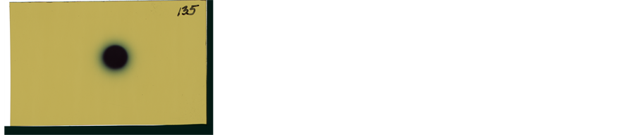
Figure 1. Full color image of EBT2 film exposed to the Sr-90/Y-90 source to a dose of 63.7 Gy. An area slightly larger than the film was scanned. The fixture that was used to position the films consistently on the scanner is visible as the dark border on two edges.
The digital image files were processed using the ImageJ image processing software [Version 1.48 g, National Institutes of Health, Bethesda] [8] . The author wrote a plug-in to perform principal component analysis, building it upon the Java Matrix Package (http://math.nist.gov/javanumerics/jama/).
The raw images were first converted to optical density by dividing each pixel by 65,535 and then negating the common logarithm of that ratio [1] [9] [10] .
 (1)
(1)
In order to determine the processing algorithm to be employed, a rectangular region of interest in the optical density image that included the source and a portion of the surrounding unexposed film in a low-dose, 0.942 Gy film was analyzed in the color dimension for its principal components. The terminology of principal component analysis is summarized in the Appendix.
The eigenimages from the principal component analysis were combined in a linear fashion to produce a processed optical density image using the equation
 (2)
(2)
where POD stands for the processed optical density, C0 is a global offset,
 ,
,
 are weighting factors and
 ,
,
 are the eigenimages from the principal component analysis. Because the principal component analysis is a linear transformation, Equation (2) may be rewritten in terms of the optical density images from each color channel as
 (3)
(3)
where is C0 a global offset,
 ,
,
 are the weights for each color channel that are derived from the principal component analysis,
 ,
,
 are the optical density images for each color channel and
 ,
,
 are separate offsets for each color channel that are the mean values of each color channel.
The mean of the intensity in a circular region of interest covering the central quarter of the area of the source in the processed optical density images was plotted as a function of dose and fit to a two-phase association curve of the form
 (4)
(4)
where POD again stands for the processed optical density, Dose is the radiation absorbed dose in gray, and F and S stand for the arbitrarily named “faster” and “slower” components respectively. This fitting was performed with the Prism statistical software package [Version 6.0d, GraphPad Software, La Jolla, CA], from which the fast and slow terminology comes. An alternative curve fitting program calls the two-phase association curve a Double Asymptotic Exponential B with Offset 2D function (http://zunzun.com).
An ImageJ processing macro was written that converts a scanned film image to optical density and computes the weighted sum of the color channels given in the previous paragraph to produce at first a processed optical density image. Then, for each pixel, it performs a binary search of the dose range from 0 to 100 Gy to find the dose that corresponds to the processed optical density of that pixel in order to produce the final image with pix- els in units of dose.
In order to validate the results of this work, a different source consisting of a 4 mm diameter by 1 mm thick vitreous disk containing 148 MBq of Y-90 was placed against the edge of a sheet of EBT2 film that had been sandwiched between two 25 mm thick blocks of polystyrene. This source was left in place for 92 seconds. This configuration and measurement were simulated in the GATE Monte Carlo simulation toolkit [Version 6.2, OpenGATE Collaboration] [11].
3. Results
A typical film image is shown in Figure 1. An area slightly larger than that of the film was scanned. The red, green and blue channels of a rectangular region of this image surrounding the source are shown in Figure 2. The red, green and blue channels were each converted to optical density and the locus of points in RGB space was plotted using the Color Inspector 3D plug-in (http://rsb.info.nih.gov/ij/plugins/color-inspector.html) to ImageJ. The full-color optical density image and the locus of those points in RGB color space are shown in Figure 3.
The principal component analysis of the region of interest yielded a mean vector of [0.334, 0.369, 0.561], ei-
genvalues of [1.04 × 10⁻⁵, 1.13 × 10⁻³, 2.45 × 10⁻¹] and an eigenvector matrix of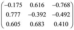 .
.
The eigenimages shown in Figure 4 were constructed by subtracting the corresponding mean value from each color channel, weighting the red, green and blue channels by the first, second and third elements respectively of a row of the matrix and adding the three weighted color channel images together to form the eigenimage for that row.
Assigning the three eigenimages arbitrarily to the red, green and blue channels, respectively, and adjusting the display window and level for low intensity pixels is shown in Figure 5 along with the trajectory of the color values of the eigenimages with that arbitrary color assignment.
Principal component analysis of a film with a dose of 0.942 Gy yielded a mean vector of [0.134, 0.170, 0.446],
eigenvalues of [1.14 × 10⁻⁶, 7.72 × 10⁻⁶, 1.48 × 10⁻³], and an eigenvector matrix of .
.
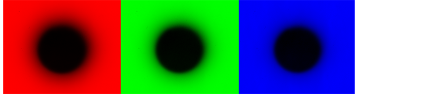
Figure 2. Red, green and blue channels (from left to right) of the central region of Figure 1. The faint irrgularity in the background of the blue channel reflects a slight nonuniformity in the thickness of the sensitive layer of the film, which is most visible in the blue channel be- cause the yellow dye most strongly absorbs blue light.
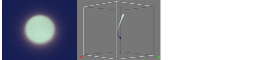
Figure 3. (Left) Full-color optical density image of a 63.7 Gy dose film; (Right) Trajectory in RGB color space of the pixels in the image to the left.
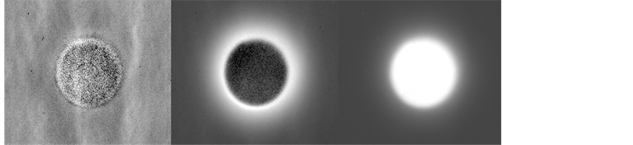
Figure 4. The three eigenimages of the image in Figure 3 corresponding, from left to right, to the three eigenvalues, from smallest to largest, and the three rows, from top to bottom, of the eigenvector matrix. The dose to this film was 63.7 Gy in the center of the source.
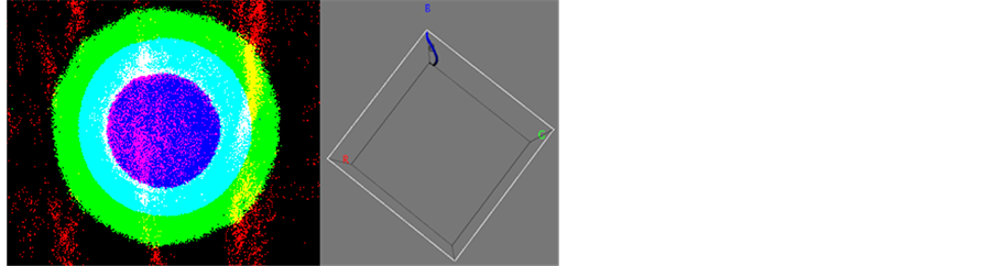
Figure 5. (Left) The three eigenimages of Figure 4 arbitrarily assigned to the red channel for the smallest eigenvalue, the green channel for the middling eigenvalue and the blue channel for the largest eigenvalue. The display has been adjusted to a low window level and a narrow width so that the colors are saturated. The transition from blue to green at the perimeter of the source demonstrates the dose-dependent color shift; (Right) The color space trajectory of the eigenimages with this arbitrary color assignment. Although these are the same data as in Figure 3 Right, after the principal component analysis, the pixels fall predominantly in the blue-green plane.
The eigenimages shown in Figure 6 were derived in the same fashion were as those in Figure 4.
The analysis of these 0.942 Gy data was used to define the transformation to create the processed optical den- sity image. Of the three eigenimages, the two with the larger eigenvalues were combined with weights of −0.574 for that with the middling eigenvalue and of 0.819 for that with the largest eigenvalue, and an offset of 0.012 was added to each pixel. These values were chosen to minimize the noise and background irregularities in the processed optical density image. This transformation of the eigenimages was then rewritten in the form of Equa- tion (3) as a weighted sum of the offset red, green and blue optical density images plus an image-wide offset given by the expression
 (5)
(5)
Note that Equation (5) writes the same transformation as the linear combination that is described at the begin- ning of this paragraph in terms of the color channels instead of the eigenimages. The transformation of the color channels in Equation (5) was subsequently applied to all of the films in order to produce monochromatic pro- cessed optical density images.
The average of the processed optical density in a circular region of interest covering the central quarter of the area of the source was analyzed as a function of dose for each of the films as shown in Figure 7.
These data were fit by the expression in the form of Equation (4)
 (6)
(6)
with an R2 value of 0.9990. The residuals of the fit are also shown in Figure 7. The standard deviation of the re- siduals was 0.00970. The maximum deviation of any processed optical density value from the fit was −0.016.
The film exposed on its edge by the second source, the 148 MBq disk of Y-90, and the corresponding Monte
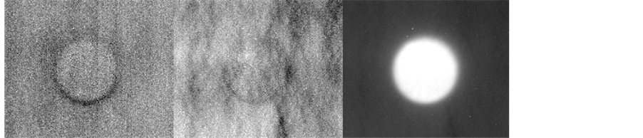
Figure 6. Eigenimages of a film with a 0.942 Gy dose. The corresponding eigenvalues range from smallest to largest from left to right in the figure.
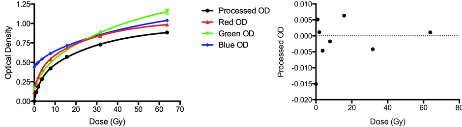
Figure 7. Optical density vs. Dose. (Left) The optical densities (OD) of the red, green and blue channels are plotted in their respective colors. The processed optical density is plotted in black. The processed optical density curve was fit to obtain the transformation from dose to processed optical density given in Equation (6); (Right) Residuals of the fit.
Carlo simulation were compared by extracting a dose profile along a line from the center of the disk at the edge of the film to a point along the normal 6 mm from the disk. The results are shown in Figure 8.
4. Discussion
The goal of this work was to develop a relatively straightforward image processing algorithm with which to convert a raw scanner image of an EBT2 film into an image of radiation absorbed dose. The approach described by the film manufacturer [1] takes into account variations in the thickness of the sensitive layer and variations across the film in the scanner performance with its “triple-channel method”. In essence, it establishes a dose- dependent trajectory in RGB color space using calibration films and then, for each RGB pixel in a measurement film, finds the nearest point on the calibration trajectory and assigns that dose to the pixel. However, the project for which the principal component-based method was developed did not require the degree of complexity and sophistication that is embodied in the commercial implementation of the triple-channel method. A free, online tool (http://radiochromic.com) implements a sophisticated algorithm [12] , but requires that the calibration films be exposed in a very specific fashion that could not be performed in the work reported here.
To calibrate the procedure reported here,
1) Convert to optical density the scanned image of a relatively low dose (around 1 Gy) radiochromic film that contains both an area that has been exposed to a known, spatially uniform dose and an area that is subject only to the effects of the nonuniformity of the sensitive layer and of scanning imperfections,
2) Perform principal component analysis of that image,
3) Construct a linear combination of the eigenimages of those principal components using weighting factors that minimize the imperfections in the unexposed region of the calibration film. The weighting factors of the li- near combination are, at present, chosen manually to minimize the visible imperfections in the unexposed re- gion,
4) Rewrite this linear combination of the eigenimages as the corresponding linear combination of the red, green and blue channels, that is, determine the parameters to be used in Equation (3),
5) Apply this transformation to a series of films that have been exposed to different known doses over the range of interest to produce processed optical density images, and
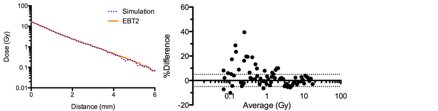
Figure 8. (Left) Comparison of the radiochromic film measurement of the dose (solid line) to the Monte Carlo simulation (broken line) as a function of distance along the central axis from the surface of a disk source of 148 MBq of Y-90; (Right) Bland-Altman plot of the percentage difference between the radiochromic film (minuend) and the Monte Carlo simu- lation (subtrahend). The horizontal axis is the average of the two values and logarithmic, thereby emphasizing the lower doses. The horizontal dotted lines represent plus and minus 5% differences.
6) Plot the processed optical densities of the uniform dose regions of these films against dose and fit those data to produce the calibration curve, that is, determine the parameters to be used in Equation (4).
To process measurement films,
1) Convert the scanned image of the film to a processed optical density image by applying Equation (3) with the parameters determined in the calibration phase to the scanned image. Then
2) Use Equation (4) with the parameters from the fit in the calibration phase to convert the processed optical density image to the dose image.
The dose-dependence of the color of the sensitive layer is illustrated in Figure 3, Figure 5 and Figure 7. Do- cumentation from the film manufacturer refers to the “spread of dose values between different channels” [10] , which presumably is a description of this effect. The dose-dependence of the color is also evident in published plots of optical density vs. dose [2] [13] and has been analyzed spectroscopically [14] .
Because of the substantial effect that the dose-dependent color shift has upon the principal components, a choice had to be made as to which set of principal components to use for the basis functions of the transforma- tion to apply to all of the scanned films, regardless of nominal dose. The principal components of any RGB im- age constitute a set of orthonormal basis functions that span the RGB feature space. Thus, it is valid to select the principal components of one image and to use them as the basis functions to decompose and then process any RGB image. A visual inspection of the eigenimages from the principal component analyses of each of the com- plete range of doses suggested that the low dose eigenvectors separate the background effects from the dose ef- fects the best. This can be seen by comparing Figure 4 and Figure 6. In Figure 4 and Figure 5, the lower dose pixels beyond the periphery of the source appear in the eigenimage with the intermediate eigenvalue (colored green in Figure 5) and the background streaks appear in the eigenimage with the smallest eigenvalue (colored red in Figure 5). In Figure 6, which has a far lower maximum dose, the dose information appears almost en- tirely in the eigenimage with the strongest eigenvalue, the background variations appear mostly in the eigeni- mage with the intermediate eigenvalue and mainly noise appears in the eigenimage with the smallest eigenvalue.
The background in the eigenimage with the strongest eigenvalue in Figure 6 includes some of the nonunifor- mities that appear strongly in the eigenimage with the middling eigenvalue. Thus, the processed optical density image was constructed from the principal component analysis of a low dose film by subtracting from the strong- est eigenimage the fraction of the middling eigenimage that minimized the nonuniformity of the background in the resulting difference image. The choice of fraction was determined by trial and error to minimize the visible nonuniformity in the background of the difference image. The eigenimage with the weakest eigenvalue, con- taining mainly what appears to be random noise, was rejected entirely, as that dimension of the feature space contains no useful information. This linear combination of eigenvectors was translated into the corresponding linear combination of color channels in Equation (3) for implementation. The means from the principal compo- nent analysis were subtracted before the weighted sum was calculated, and a small constant was added to make the average value of the background pixels well away from the region of the source be nil. Because these are all linear transformations, the linear combination of eigenimages can be rewritten as a linear combination of the color channels’ offset optical density images. This transformation was applied to all of the films in order to pro- duce the processed optical density images. This transformation can be viewed as a shift in color space to the center of the cloud of feature vectors followed by a rotation to align the trajectory of pixel colors with one of the axes. Then, each processed optical density image represents the projection of its original RGB data translated and then projected onto that rotated axis.
Note that principal component analysis has been used only to define the transformation of the red, green and blue channels into the processed optical density image. It was performed during the design of the algorithm in order to isolate the different characteristics (roughly speaking noise, background variations and dose) of each image and to facilitate designing a transformation that minimizes the undesirable characteristics in the final im- age. If one assumes that the noise is uniformly distributed in the color space and that the background intensity variations are not a function of the dose of the source, then the selected transformation eliminates the same amounts of noise and of the background variations regardless of the dose of the source. What differs is that a small portion of the dose-related density will be lost at higher dose levels because of the dose-dependent color shift. However, the mapping from processed optical density to dose takes that into account along with the gener- al saturation effect.
The processed optical density curve has a dynamic range that is greater than those of the red and blue chan- nels and nearly that of the green channel. The mapping from processed optical density in the region of interest at the center of the source to the nominal dose in that region is fit well by the sum of two association curves or ex- ponential buildup curves in Equation (4). This fitting function was chosen empirically, but it is similar in form to Equation 19 of del Moral, et al. [15] .
Ideally, this functional fit would be inverted analytically to give an expression for the dose as a function of the processed optical density. The author could not derive such an expression, so a binary search of possible doses for the processed optical density of each pixel was performed by repeatedly solving the fitted expression for progressively better refined estimates of the dose. This searching method runs quickly on a personal computer, taking about two seconds to process an image with half a million pixels. As a practical matter, the maximum dose for the search was set to 100 Gy, since by that dose, the curve is so close to horizontal that its slope greatly amplifies relatively small differences in the processed optical density.
A substantial amount of time between exposure and scanning was necessary for logistical reasons. The cali- bration films were exposed at the end of the working day 70 km from where they were to be scanned and thus an appreciable number of films were accumulated for later scanning. A delay of two days’ duration, nominally 48 hours, was used so that the films would have self-developed to 97% or more of their ultimate densities and a variation of a few hours in the length of the delay would have a negligible effect upon the scanned measure- ments [1] [10] [16] .
ImageJ was chosen as the foundation of this work because it is freely available, runs on a wide variety of computers, has a rich set of intrinsic features and is easily extensible using its own macro language as well as the freely available Java programming language. There are a number of optional modules (called “plug-ins”) that one can obtain for ImageJ to perform principal component analysis. However, none of them provided all of the features that were required by this project. The requisite features of the principal component analysis plug-in that was written for this project were the definition of a region of interest within the image in which to calculate the principal components just of that region, and the synthesis of an image from a weighted sum of the eigeni- mages that arise from that analysis. An ImageJ macro was written to automate the conversion of a raw scanned image first into an optical density image, thence into a monochromatic optical density image and finally into a dose image based on the experimentally-derived calibration curve.
The generally close agreement between radiochromic film measurements processed by the method described here and the dose predicted by the Monte Carlo simulation shown in Figure 8 demonstrates the validity of this method. The Bland-Altman plot illustrates the rather large percentage differences between the radiochromic film measurement and the simulation at very low doses. These are seen to be due to imperfections in the simulation at those low doses. These imperfections vary when different seed values are used in the random number genera- tor of the simulation.
The precise values of the transformation parameters that were employed in this work might not be generally applicable beyond the type of radiation, the lot of EBT2 film, the particular scanner and the aging time that were employed in this study. The sensitivity of the transformation parameters to variations in these conditions re- mains to be investigated.
5. Conclusion
A transformation of the red, green and blue channels of a digital scan of EBT2 radiochromic film to dose has been developed based upon a principal component analysis to separate noise and background variations in the density of the film from the dose response of the film and a nonlinear mapping of the processed optical density data to dose. It has been demonstrated to work well from 0 to 16 Gy.
Acknowledgements
The author gratefully acknowledges the support of this work by a contract from LV Liberty Vision Corporation and by IsoTherapeutics Group, LLC.; the advice of William D. Erwin, M.S., Firas Mourtada, Ph.D., David S. Followill, Ph.D., Ann A. Lawyer, M.S., David T. Fuentes, Ph.D., and anonymous reviewers; and the assistance of Prakash Bakhru, M.S., and the M.D. Anderson Radiation Safety Office. The author thanks the creators of the various free software packages that were used in this work.
References
- Micke, A., Lewis, D.F. and Yu, X. (2011) Multichannel Film Dosimetry with Nonuniformity Correction. Medical Physics, 38, 2523-2534. http://dx.doi.org/10.1118/1.3576105
- Lewis, D., Micke, A., Yu, X. and Chan, M.F. (2012) An Efficient Protocol for Radiochromic Film Dosimetry Com- bining Calibration and Measurement in a Single Scan. Medical Physics, 39, 6339-6350. http://dx.doi.org/10.1118/1.4754797
- Sim, G.S., Wong, J.H.D. and Ng, K.H. (2013) The Use of Radiochromic EBT2 Film for the Quality Assurance and Dosi- metric Verification of 3D Conformal Radiotherapy Using Microtek Scan Maker 9800XL Flatbed Scanner. Journal of Applied Clinical Medical Physics, 14, 85-95. http://dx.doi.org/10.1120/jacmp.v14i4.4182
- Hotelling, H. (1933) Analysis of a Complex of Statistical Variables into Principal Components, Part 1. Journal of Educational Psychology, 24, 417-441. http://dx.doi.org/10.1037/h0071325
- Hotelling, H. (1933) Analysis of a Complex of Statistical Variables into Principal Components, Part 2. Journal of Edu- cational Psychology, 24, 498-520. http://dx.doi.org/10.1037/h0070888
- Wintz, P.A. (1972) Transform Picture Coding. Proceedings of the IEEE, 60, 809-820. http://dx.doi.org/10.1109/PROC.1972.8780
- Gonzalez, R.C. and Woods, R.E. (2008) Digital Image Processing. 3rd Edition, Pearson Prentice Hall, Upper Saddle River.
- Schneider, C.A., Rasband, W.S. and Eliceiri, K.W. (2012) NIH Image to ImageJ: 25 Years of Image Analysis. Nature Methods, 9, 671-675. http://dx.doi.org/10.1038/nmeth.2089
- Butson, M.J., Yu, P.K., Cheung, T. and Metcalfe, P. (2003) Radiochromic Film for Medical Radiation Dosimetry. Materials Science and Engineering: R: Reports, 41, 61-120. http://dx.doi.org/10.1016/S0927-796X(03)00034-2
- International Specialty Products (2010) Gafchromic EBT2 Self-Developing Film for Radiotherapy Dosimetry, Revision 3. International Specialty Products, Wayne. http://www.filmqapro.com/Documents/GafChromic_EBT-2_20101007.pdf
- Jan, S., Santin, G., Strut, D., et al. (2004) GATE: A Simulation Toolkit for PET and SPECT. Physics in Medicine and Bio- logy, 49, 4543-4561. http://dx.doi.org/10.1088/0031-9155/49/19/007
- Mendez, I., Peterlin, P., Hudej, R., Strojnik, A. and Casar, B. (2014) On Multichannel Film Dosimetry with Channel- Independent Perturbations. Medical Physics, 41, Article ID: 011705. http://dx.doi.org/10.1118/1.4845095
- Devic, S., Tomic, N., Soares, C.G. and Podgorsak, E.B. (2009) Optimizing the Dynamic Range Extension of a Radio- chromic Film Dosimetry System. Medical Physics, 36, 429-437. http://dx.doi.org/10.1118/1.3049597
- Devic, S., Tomic, N., Pang, Z., et al. (2007) Absorption Spectroscopy of EBT Model GAFCHROMICTM Film. Medical Physics, 34, 112-118. http://dx.doi.org/10.1118/1.2400615
- Del Moral, F., Vazquez, J.A., Ferrero, J.J., et al. (2009) From the Limits of the Classical Model of Sensitometric Curves to a Realistic Model Based on the Percolation Theory for GafChromic EBT Films. Medical Physics, 36, 4015-4026. http://dx.doi.org/10.1118/1.3187226
- Arjomandy, B., Tailor, R., Anand, A., et al. (2010) Energy Dependence and Dose Response of Gafchromic EBT2 Film over a Wide Range of Photon, Electron and Proton Beam Energies. Medical Physics, 37, 1942-1947. http://dx.doi.org/10.1118/1.3373523
- Bruyant, P.P., Sau, J. and Mallet, J.-J. (1999) Noise Removal Using Factor Analysis of Dynamic Structures: Applica- tion to Cardiac Gated Studies. Journal of Nuclear Medicine, 40, 1676-1682.
- Wendt III, R.E., Erwin, W.D. and Groch, M.W. (2000) Principal Component Analysis of Multigated Cardiac Blood- pool Studies and Correction of Count-deficient Frames. Proceedings of the 13th IEEE Symposium on Computer-Based Medical Systems, IEEE Computer Society, Houston, 195-200. http://dx.doi.org/10.1109/CBMS.2000.856899.
Appendix
To summarize the notation and concepts of principal component analysis, consider a full color image to be a three-dimensional dataset that has the width and height of the image and a thickness of three in the color direc- tion. Each pixel,
 , is a vector of length three, consisting of the red, green and blue channels of the color im- age,
 . The index i ranges over the pixels in the region of analysis within the image.
The mean vector consists of the means of each color channel
 (7)
(7)
where N is the number of pixels in the region of analysis within the image.
The covariance matrix of the pixels
 (8)
(8)
contains the information about how each dimension of the image (i.e., each of the three color channels) varies with respect to the others. Because
 is real and symmetric it is possible to transform it into a matrix,
 , whose off-diagonal elements are zero, meaning that the transformed feature space has indepen- dent dimensions (whereas the original red, green and blue channels are likely to be correlated to some degree and hence dependent). The diagonal elements of
 are the eigenvalues of
 . The rows of the transforma- tion matrix A are the eigenvectors of the transformed space and thus form a set of orthonormal basis functions that span the feature space. The A and
 matrices are computed by the “Eigenvalue Decomposition” class of the Java Matrix Package (http://math.nist.gov/javanumerics/jama/). The relative magnitudes of the eigenvalues indicate how much of the variation among pixels in the image occurs along the direction of the corresponding eigenvectors. The eigenimages (e.g., Figure 4 and Figure 6) are the components of the transformed image
 .
.
It is possible to represent the original pixels by . An approximation to the original image may be reconstructed from a subset of the eigenvectors,
 , where
 , that is, from a subspace of the transformed feature space.
This type of approximation in which eigenvectors that bear little information have been discarded has been used for noise reduction [17] [18] . For the principal components used in this work, the eigenvector with the weakest eigenvalue was completely eliminated from the reconstruction for this reason, as the corresponding ei- genimage appears to be predominantly of noise. In the present application, it was also desired to minimize the inhomogeneity of the background that arises in part from the irregularity in the thickness of the sensitive layer. That inhomogeneity was visible in both of the remaining eigenimages. Thus, the particular combination of the eigenimages was chosen to minimize the visible irregularity in the background as well as to eliminate some noise.