J. Biomedical Science and Engineering, 2011, 4, 341-351
doi:10.4236/jbise.2011.45043 Published Online May 2011 (http://www.SciRP.org/journal/jbise/
JBiSE
).
Published Online May 2011 in SciRes. http://www.scirp.org/journal/JBiSE
Comparison of ICA and WT with S-transform based method
for removal of ocular artifact from EEG signals
Kedarnath Senapati1, Aurobinda Routray2
1Institute of Mathematics and Applications, Bhubaneswar, India;
2Department of Electrical Engineering, Indian Institute of Technology, Kharagpur, India.
Received 11 February 2011; revised 11 March 2011; accepted 7 April 2011.
ABSTRACT
Ocular artifacts are most unwanted disturbance in
electroencephalograph (EEG) signals. These are
characterized by high amplitude but have overlap-
ping frequency band with the useful signal. Hence, it
is difficult to remove the ocular artifacts by tradi-
tional filtering methods. This paper proposes a new
approach of artifact removal using S-transform (ST).
It provides an instantaneous time-frequency repre-
sentation of a time-varying signal and generates high
magnitude S-coefficients at the instances of abrupt
changes in the signal. A threshold function has been
defined in S-domain to detect the artifact zone in the
signal. The artifact has been attenuated by a suitable
multiplying factor. The major advantage of ST-fil-
tering is that the artifacts may be removed within a
narrow time-window, while preserving the frequency
information at all other time points. It also preserves
the absolutely referenced phase information of the
signal after the removal of artifacts. Finally, a com-
parative study with wavelet transform (WT) and in-
dependent component analysis (ICA) demonstrates
the effectiveness of the pr oposed approach.
Keywords: EEG, Ocular Artifact; S-Transform;
Wavelet Transform; Independent Component Analysis
1. INTRODUCTION
Electroencephalogram (EEG) is the recorded electric
potential from the exposed surface of the brain or from
the outer surface of the head. The raw EEG data is con-
taminated with numerous high and low frequency noise
known as artifacts. High frequency noise is a result of
atmospheric thermal noise and power frequency noise.
Low frequency noise is primarily caused by eye move-
ments, respiration and heart beats. Such artifacts are
characterized by amplitude in the millivolt range (whereas
the actual EEG is in microvolt range) in the frequency
band of 0 - 16 Hz [1].
The presence of these artifacts in the raw EEG poses a
major problem to researchers. Various methods to re-
move such artifacts have been proposed in the literature.
These methods include Principal Component Analysis
(PCA), Independent Component Analysis (ICA) and
wavelet based thresholding. Croft and Barry [2] and
Kandaswamy et al. [3] reviewed several methods of ar-
tifact removal. Lagerlund et al. [4] use a Principal
Component Analysis (PCA) based filtering of EEG sig-
nal for artifact removal. Therefore, a major drawback of
the PCA method is that it cannot completely separate
ocular artifacts from EEG signals, when both waveforms
have similar voltage magnitudes. Decomposition into
uncorrelated signal components is possible with PCA;
however, it is not sufficient to produce independence
between the variables, at least when the variables have
non-Gaussian distributions. The PCA method therefore
cannot accommodate higher-order statistical dependen-
cies.
Jung et al. [5], Delorme et al. [6] and LeVan [7] de-
veloped some artifact removal techniques using ICA
which demonstrates the potential not only to decorrelate
but also to work with higher-order dependencies. The
most significant computational difference between ICA
and PCA is that PCA uses only second-order statistics
(such as the variance which is a function of the data
squared) while ICA uses higher-order statistics (such as
functions of the data raised to the fourth power). Vari-
ables with a Gaussian distribution have zero statistical
moments above second-order, but most signals do not
have a Gaussian distribution and do have higher-order
moments. These higher-order statistical properties are
put to good use in ICA. While ICA is an extension of
PCA method, these component-based artifact removal
procedures are not automated and require tuning of sev-
eral parameters such as number of sources, permutation
of these sources etc. through visual inspection.
Krishnaveni et al. [1] recently proposed a wavelet

K. Senapati et al. / J. Biomedical Science and Engineering 4 (2011) 341-351 342
based thresholding method to remove ocular artifacts
from raw EEG data. Kumar et al. [8] developed a similar
wavelet based statistical method for removing ocular
artifacts. The wavelet based artifact removal techniques
are notable for preserving the shape of the waveform of
the signal in the artifact free zone compared with other
artifact removal methods. But this method is limited by
the introduction of noise beyond the specified frequency
band when applied to band limited signals.
In this paper the authors propose a new method of
ocular artifact removal from EEG signal using the
S-transform [9,10]. The high amplitude signal compo-
nents, like the ocular artifacts are filtered out in
S-domain by setting a statistical threshold function. The
ST based method is an improvement of the wavelet
method since it localizes the power and preserves the
absolutely referenced phase information of the original
signal. Moreover, integrating the S-transform over time,
results in the Fourier transform (FT). This direct relation
to the Fourier transform simplifies the task of inverting
to the time domain. This property of the S-transform led
to the development of S-transform filter, which has been
explored in this work to serve the purpose of removing
ocular artifacts.
The paper has been organized as follows. The meth-
odology used for signal preprocessing and artifact re-
moval using ICA, WT and S-transform is described in
Section 2. Results and discussions are contained in Sec-
tion 3 followed by the conclusions in Section 4.
2. METHODOLOGY
The methodology involves pre-filtering followed by the
application of various methods such as ICA, wavelet and
S-transform as discussed below.
2.1. Filtering
As discussed above the raw EEG data is contaminated
with high frequency noises other than ocular artifacts.
The signal is passed through a low pass filter with cutoff
frequency of 30 Hz followed by normalization. Nor-
malization ensures removal of any unwanted bias that
may have crept into the experimental recordings. These
normalized signals have been used further for artifact
removal.
2.2. Independent Component Analysis
Independent component analysis is a powerful technique
which can be used to separate sources from a given lin-
ear mixture of signals. The brain is supposed to have
many independent sources which produce electrical sig-
nals. The EEG signal that is obtained by various elec-
trodes actually contains a linear mixture of the signals
produced by independent sources in the brain. In a signal
having artifacts the linear mixture also contains the sig-
nals produced by ocular and other visceral sources. If we
are able to separate the sources from the signals recorded
by the various electrodes we can easily identify the arti-
fact sources and can separate them from the original
EEG sources. Once the independent time courses of dif-
ferent brain and artifact sources are extracted from the
data, “corrected” EEG signals can be derived by elimi-
nating the contributions of the artifactual sources. The
method described here basically tries to separate and
eliminate the ocular sources. Subsequently the linear
mixture is reconstructed using the artifact free sources.
This linear mixture is then called the artifact free signal.
The signal obtained from the electrodes can be ex-
pressed in the following manner
.

xAs (1)
Here
 
12
,,, T
m
x
kxk xk




x
1m

12
is called the
observation vector. The observation vector in our case is
composed of the signals obtained from the electrodes.
The observation vector has () components. The
source vector is given by
 
,,, T
n
s
kss
1n
k sk


;
it gives the different independent sources which results
in observation vector after linear mixing. The source
vector has (

) components and they are assumed to
be statistically independent; and that they are
non-Gaussian. A is called the mixing matrix composed
of (mn

) constant elements ij . This matrix gives the
linear transformation between the source vector and the
observation vector.
a
The independent component analysis problem is for-
mulated as finding a demixing or separating matrix W
from the given observation matrix x, such that
.

yWx (2)
here
 
12
,,, T
n
yk ykyk




y is the estimate of
original source vector s and the components i are as
independent as possible. This can be achieved by maxi-
mizing some function
y


,
n12
,,
F
yy
mn
y that measures
independence. The various approaches differ in the spe-
cific objective function and the optimization method that
is used. There are certain basic assumptions in the prob-
lem formulation. Firstly the number of observed signals
should be equal to the number of independent sources,
i.e.,

. Therefore A represents a full rank square
mixing matrix. This is not really a restriction since PCA
can always be applied to reduce the dimension of the
data set x, to equal that of the source data set s. Another
assumption is that source signals must be statistically
independent of each other or in practice as independent
as possible (including uncorrelatedness). The independ-
ence condition can be defined by stating that the joint
probability density of the source signals is equal to the
product of the marginal probability densities of the indi-
C
opyright © 2011 SciRes. JBiSE

K. Senapati et al. / J. Biomedical Science and Engineering 4 (2011) 341-351 343
kvidual signals, i.e.,
 
1
.
n
i
i
ppy




y
Two categories of ICA algorithm exist. In the first
type, source separation can be obtained by optimizing an
objective function [11] which can be scalar measure of
some distributional property of the output y. More gen-
eral measures are entropy, mutual independence, diver-
gence between joint distribution of y and some given
mode and higher order decorrelation.
The ICA method can be formulated as optimization of
a suitable objective function which is also termed as
contrast function. The problem in optimization of con-
trast function is that, they rely on batch computation
using the higher order statistics (HOS) of data or lead to
complicated adaptive separation. It is often sufficient to
use simple HOS such as kurtosis, which is the fourth
order cummulant with zero time lags. The kurtosis of the
source signal
th
ii
s
is given by
 
2
44 2
Cum 3
ii i
sEs Es



 

(3)
If i
s
is Gaussian, then its kurtosis is zero. Source
signals that have negative kurtosis are called sub-Gaus-
sian and have a probability distribution flatter than usual
Gaussian distribution. Source signals having a positive
kurtosis are called super-Gaussian and have a probability
distribution with sharp peak and longer tails then the
standard Gaussian ones. A contrast function based on
kurtosis is given by

 
2
44
1
11
Cum 3
nn
ii
ii
JyEy Ey




 

y2
i
(4)
where stands for cummulant. It is maximized by
a separating matrix W, if the sign of the kurtosis is same
as all the source signals. For pre-whitened input vector x
and orthogonal separating matrices,
Cum
21
i
Ey


 and
hence the contrast function


1
Jy reduces to 2
i
Ey 3





4
n
.
Therefore, is maximized when

1
Jy
1
i
i
Ey





 is
minimized for sources having negative kurtosis and
maximized for sources with positive kurtosis.
The second category uses neural implementation of
ICA algorithms like non-linear PCA based subspace
learning [12,13] for achieving source separation. In this
category, there are adaptive algorithms [13] like mini-
mum mutual information method [14] and maximum
entropy method [15] based on stochastic gradient opti-
mization. An excellent treatment of the various ap-
proaches, their strengths and weaknesses can be found in
Cichicki et al. [16], as well as Hyvärinen et al. [17].
The method that has been used in this study is based
on minimization of mutual information between outputs
which is equivalent to maximization of their joint en-
tropy. The details of the algorithm which is known as
infomax principle can be found in [18].
In this study we have used 19 electrodes to collect
EEG data from a human subject. Hence exactly 19 in-
dependent components (sources) can be separated out
using infomax based ICA, from the observed recordings
(mixtures). Out of these 19 sources, the sources contain-
ing ocular artifacts can be identified and removed and
subsequently artifact free signals are obtained recon-
structing from the rest of the components.
2.3. Artifact Removal Using Wavelet Transform
Wavelet transform is a useful tool for time frequency
analysis of neurophysiological signals. Wavelets are
small wave like oscillating functions that are localized in
time as well as in frequency [19,20]. In discrete domain,
any finite energy time domain signal can be decomposed
and expressed in terms of scaled and shifted versions of
a mother wavelet


t  and a corresponding scaling
function


t

. The scaled and shifted version of the
mother wavelet is mathematically represented as




/2
,22, ,
jj
jk ttkj
 kZ


(5)
A similar expression holds for , the scaled and
shifted version of the scaling function

,jk t


t

.
A signal


ht can be expressed mathematically in
terms of the above wavelets at level as j



 


,,jjkj jk
kk
hta ktdkt  

 (6)
where


j
ak and


j
dk are the approximate and
detailed coefficients at level . These coefficients are
computed using filter bank approach as proposed by
Rioul and Vetterli [21].
j
The original signal


ht is first passed through a
pair of high pass and low pass filters. The low frequency
component approximates the signal while the high fre-
quency components represent residuals between original
and approximate signal. The approximate component is
further decomposed at successive levels. The output time
series is down-sampled by two and then fed to next level
of input after each stage of filtering.
As the wavelet coefficients represent the correlation of
signal with the mother wavelet, the signal will generate
high amplitude coefficients at places where artifacts are
present. These coefficients can be eliminated using a
simple thresholding technique. The threshold can be
computed as


2
jj
TmeanC stdC

.
j
(7)
here
j
C is the wavelet coefficient at level of de-
composition. If the value of any coefficient is greater
than the threshold it is reduced to a suitable fraction of
th
j
C
opyright © 2011 SciRes. JBiSE

K. Senapati et al. / J. Biomedical Science and Engineering 4 (2011) 341-351 344
the actual coefficient value [8].
2.4. S-Transform
The S-transform provides a useful extension to the
wavelets by having a frequency dependent progressive
resolution as opposed to the arbitrary dilations used in
wavelets. The kernel of the S-transform does not trans-
late with the localizing window function, in contrast to
the wavelet counterpart. For that reason the S-transform
retains both the amplitude and absolutely referenced
phase information [9]. Absolutely referenced phase in-
formation means that the phase information given by the
S-transform is always referenced to time . This is
the same meaning of the phase given by the Fourier
transform, and is true for each S-transform sample of the
time-frequency space. The wavelet transform (WT), in
comparison can only localize the amplitude or power
spectrum, not the absolute phase. There is, in addition,
an easy and direct relation between the S-transform and
the natural Fourier transform which cannot be achieved
by wavelets. Since its development, the S-transform has
been widely used in applications ranging from geophys-
ics [10], oceanography [22], atmospheric physics [9,23-
25], medicine [26,27], hydrogeology [28] and mechani-
cal engineering [29].
0t
The S-transform of a continuous time signal


ht is
defined as [30,31]
 
2π
,,
ift
Sfhtw tft 



ed. (8)
The window function w, is generally chosen to be
positive and normalized Gaussian [25]


22
2
,e
2π
tf
f
wtf




 (9)
where f represents the frequency, t is the time and

is
the delay. It is worth emphasizing that in order to have
an inverse S-transform, the window must be normalized

,d1wtf t


.

 (10)
The S-transform can also be written as the convolution
of two functions over the variable t
 

,,,
,,
Sfptfw tf
pfwf






dt
(11)
where



2π
,e
if
pfh



 (12)
and

22
2
,e
2π
f
f
wf



 (13)
Let


,Bf  be the Fourier transform (from

to

) of the S-transform . By the convolution
theorem the convolution in the

,Sf 


(time) domain be-
comes a multiplication in the

(frequency) domain:



 
,,,BfPfWf  . (14)
Here


,Pf  and


,Wf  are the Fourier trans-
forms of


,pf  and


,wf  respectively. Equation
(14) can also be written as
 
22
2
2π
,f BfH fe



 (15)
where


H
f 

is the Fourier transform of (12) and
the exponential term is the Fourier transform of the
Gaussian function (13). Thus the S-transform can be
retrieved by applying the inverse Fourier transform (

to

) to the above equation for , 0f



 



22
2
1
2π
2π
,,
eed
f
SfHfW f
Hf



.









(16)
One of the important characteristics of the S-transform
is that summing


,Sf  over

yields the Fourier
spectrum of the signal h. Using the definition (8) of
S-transform we obtain
 
2π
,e dd
ft
H
fhtwtft


 
 

 (17)
where


H
f is the Fourier transform of


ht . If


Hf

, applying Fubini’s theorem and taking into
account the normalization condition (10), the above
equation reduces to a simple Fourier transform
 
,dHfS f.




 (18)
This spectral property enables the definition of an in-
verse S-transform through the inverse Fourier transform.
Thus
 
2π
,ded.
ift
htS ff 

 



 (19)
This is clearly different from the concept of wavelet
transform. The S-transform can be written as operations
on the Fourier spectrum


H
f of


ht.
 
22
2
2π
2π
,eed
i
f
SfH ff


 


0.


 (20)
The discrete analog of (20) is used to compute the
C
opyright © 2011 SciRes. JBiSE

K. Senapati et al. / J. Biomedical Science and Engineering 4 (2011) 341-351 345
discrete S-transform by taking advantage of the Fast
Fourier Transform (FFT) and the convolution theorem.
Using (13), the S-transform of a discrete time series
is given by (letting

hkT
f
nNT and jT

)
22
2
2π2π
1
0
,ee
mimj
NnN
m
nmn
SjT Hn
NT NT







0
(21)
and for it is equal to the constant defined as 0,n

1
0
1
,0
N
m
m
SjTh
NNT







(22)
where and The discrete in-
verse of S-transform [9] is given by
,jm0,1, ,1.nN

2π
11
00
1,e
ink
NN N
nj
n
hkTS jT
NNT








 .
(23)
The amplitude of the S-transform has the same mean-
ing as the amplitude of the Fourier transform. This pro-
vides a frequency invariant amplitude response in con-
trast to the wavelet approach [31]. The term “frequency
invariant amplitude response” means that for a sinusoi-
dal signal with amplitude
 


00
cos 2π
A
ht Aft
0
, the
S-transform returns amplitude
A
regardless of the
frequency f.
2.5. Artifact Removal Using S-Transform
When only single channel signal is available, component
based methods like PCA and ICA cannot be applied. In
such case, the use of S-transform has been demonstrated
to be an important tool to remove ocular artifacts from
EEG signals, since it not only solves the task efficiently
but also retains the local phase information of the origi-
nal signal even after denoising. The following is a sum-
mary of the proposed algorithm.
1) Decompose the entire EEG signal using S-trans-
form.
2) Select the frequency band


0, 1 6
H
z, where, gen-
erally the ocular artifacts lie.
3) Determine the mean and standard deviation of the
absolute values of S-transform coefficients


,Sij in
the selected frequency band.
4) Set the threshold function as:




mean,2*std,,TSij Si

jwhere


,Sij

is the absolute value of .

,Sij
5) Set the multiplying factor .
01mf
6) If

,Sij T, then, , else
.

,Sij Si

,*j mf
 
,,Sij Sij

7) Reconstruct the signal using the modified S-trans-
form coefficients.
High amplitude S-transform coefficients are generated
at the places where artifacts are present. These coeffi-
cients are eliminated by using the above threshold tech-
nique. The time average of the local spectral representa-
tion (i.e., the S-transform) is the complex-valued global
Fourier spectrum as in (18). As a result, the ST can be
interpreted as a generalization of Fourier transform to a
nonstationary signal. Since the EEG signal is highly
nonstationary, the S-transform is the ideal method for
representing its time-frequency distribution. It is also
customary in Fourier spectra to show only the positive
frequency part of the spectrum, because the amplitude
spectrum is symmetric, and the phase spectrum is anti
symmetric. However, any operation (here, thresholding)
in the S-domain must be applied to both the positive and
negative frequency parts of the spectrum. Otherwise, the
summed ST will not collapse to FT. When any operation
is applied to the positive or negative part of the spectrum
only, the inverse FT leads to a complex (not real) time
series, and would be in error.
Here, signal reconstruction performance is measured
by the signal-to-noise ratio (SNR) and is defined by
2
2
10
20log l
rec l
h
SNR hh  (24)
where h and rec h represent the original and recon-
structed signal respectively.
3. RESULT AND DISCUSSIONS
In this paper we have evaluated the performance of the
proposed denoising method using S-transform to remove
ocular artifacts from EEG signal with respect to the ICA
and wavelet based method discussed in Section II. The
Figures related to ICA presented in this paper are pro-
duced using the EEGLAB software package which op-
erates in the MATLAB environment and available at
http://sccn.ucsd.edu/eeglab.
In Figure 1, the removal of ocular artifacts from EEG
signals collected from multiple sensors is demonstrated.
A five-second epoch of raw EEG time series containing
prominent artifact due to eye movement is shown in
Figure 1(a). First, the raw 19-channel EEG data are de-
composed into nineteen independent components using
ICA based on infomax principle (Figure 1(b)). As ex-
pected, correlation between ICA traces are close to zero.
The 2-D scalp component map of all nineteen ICs is
illustrated in Figure 1(c). Since the EEG spectrum of
eye artifacts decreases smoothly, their scalp topogra-
phies look like component 1. This artifactual component
is also relatively easy to identify by visual inspection of
component time course (Figure 1(b)). Since this com-
ponent accounts for eye activity, we may wish to sub-
tract it from the data. After removing component 1 we
reconstruct the data using the rest 18 components in or-
der to get ocular artifacts free EEG signals which is
shown in Figure 1(d).
C
opyright © 2011 SciRes. JBiSE

K. Senapati et al. / J. Biomedical Science and Engineering 4 (2011) 341-351 346
(a)
(b)
(c)
(d)
Figure 1. Demonstration of ocular artifact removal using ICA in EEG signals. (a) A
five-second epoch of a nineteen-channel EEG time series containing prominent arti-
fact due to eye movement; (b) Corresponding ICA component activations and (c)
scalp map of all the nineteen ICs; (d) Ocular artifact-free EEG signals by removing
component 1 in (b).
JBiSE

K. Senapati et al. / J. Biomedical Science and Engineering 4 (2011) 341-351 347
ICA decomposition is possible only for multi channel
data and hence cannot be applied when the data is avail-
able in single channel. Therefore the proposed S-trans-
form technique is effectively applied in order to remove
artifacts from single channel signal. A raw EEG signal of
8 sec duration sampled at 256 Hz and its S-transform is
shown in Figure 2(a). Using infomax based ICA method,
ocular artifacts are removed from all the nineteen channel
EEG signals and the exact segment of the signal (Figure
2(b)) that has been used for WT and ST study also is
taken for comparison. It can be observed in Figure 2(b),
that the high amplitude ocular artifacts are significantly
reduced in the reconstructed signal but its S-transform
plot reveals that the time-frequency distribution as com-
pared to the original signal is massively disturbed which
implies substantial loss in data in the useful signal outside
the artifact range. In Figure 2(d), the time frequency plot
after thresholding the S-coefficients and the correspond-
ing reconstructed signal are illustrated. The S-coefficients
in the range of 0.5 - 16 Hz have been subjected to thresh-
olding since most artifacts lie within this band of signal.
It can be observed in the Figure 2(d), that the high am-
plitude ocular artifacts in the specified band are signifi-
cantly reduced in the reconstructed signal. In addition,
the reconstructed signal retains all other amplitudes and
frequencies as well, of the signals. This is also apparent
in the corresponding ST plot and can be explained by the
“frequency invariant amplitude response” property of
S-transform. The artifact removed signal using wavelet
transform and its corresponding time frequency repre-
sentation using S-transform is demonstrated in Figure
2(c). This time-frequency plot contains some unwanted
frequency components beyond the actual frequency range
of the signal.
A comparison of the power spectral density (PSD) of
the raw signal and the reconstructed signal is shown in
Figure 3. The PSD of S-transform based reconstructed
signal almost replicates the PSD of the raw signal be
Figure 2. (a) Normalized raw EEG signal; (b) Artifact free EEG signal using ICA; (c) Artifact free EEG signal using wavelet trans-
form; (d) Artifact free EEG signal using S-transform. The figures in the right side are the corresponding time-frequency plot using
S-transform, of the signals in the left.
C
opyright © 2011 SciRes. JBiSE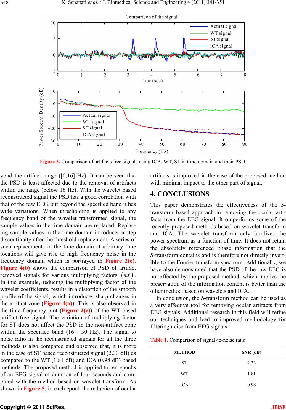

K. Senapati et al. / J. Biomedical Science and Engineering 4 (2011) 341-351 348
Figure 3. Comparison of artifacts free signals using ICA, WT, ST in time domain and their PSD.
yond the artifact range ([0,16] Hz). It can be seen that
the PSD is least affected due to the removal of artifacts
within the range (below 16 Hz). With the wavelet based
reconstructed signal the PSD has a good correlation with
that of the raw EEG, but beyond the specified band it has
wide variations. When thresholding is applied to any
frequency band of the wavelet transformed signal, the
sample values in the time domain are replaced. Replac-
ing sample values in the time domain introduces a step
discontinuity after the threshold replacement. A series of
such replacements in the time domain at arbitrary time
locations will give rise to high frequency noise in the
frequency domain which is portrayed in Figure 2(c).
Figure 4(b) shows the comparison of PSD of artifact
removed signals for various multiplying factors


mf .
In this example, reducing the multiplying factor of the
wavelet coefficients, results in a distortion of the smooth
profile of the signal, which introduces sharp changes in
the artifact zone (Figure 4(a)). This is also observed in
the time-frequency plot (Figure 2(c)) of the WT based
artifact free signal. The variation of multiplying factor
for ST does not affect the PSD in the non-artifact zone
within the specified band (16 - 30 Hz). The signal to
noise ratio in the reconstructed signals for all the three
methods is also compared and observed that, it is more
in the case of ST based reconstructed signal (2.33 dB) as
compared to the WT (1.81 dB) and ICA (0.98 dB) based
methods. The proposed method is applied to ten epochs
of an EEG signal of duration of four seconds and com-
pared with the method based on wavelet transform. As
shown in Figure 5, in each epoch the reduction of ocular
artifacts is improved in the case of the proposed method
with minimal impact to the other part of signal.
4. CONCLUSIONS
This paper demonstrates the effectiveness of the S-
transform based approach in removing the ocular arti-
facts from the EEG signal. It outperforms some of the
recently proposed methods based on wavelet transform
and ICA. The wavelet transform only localizes the
power spectrum as a function of time. It does not retain
the absolutely referenced phase information that the
S-transform contains and is therefore not directly invert-
ible to the Fourier transform spectrum. Additionally, we
have also demonstrated that the PSD of the raw EEG is
not affected by the proposed method, which implies the
preservation of the information content is better than the
other method based on wavelets and ICA.
In conclusion, the S-transform method can be used as
a very effective tool for removing ocular artifacts from
EEG signals. Additional research in this field will refine
our techniques and lead to improved methodology for
filtering noise from EEG signals.
Table 1. Comparison of signal-to-noise ratio.
METHOD SNR (dB)
ST 2.33
WT 1.81
ICA 0.98
C
opyright © 2011 SciRes. JBiSE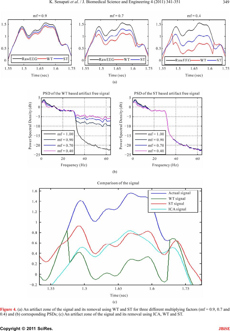

K. Senapati et al. / J. Biomedical Science and Engineering 4 (2011) 341-351 349
(a)
(b)
(c)
Figure 4. (a) An artifact zone of the signal and its removal using WT and ST for three different multiplying factors (mf = 0.9, 0.7 and
0.4) and (b) corresponding PSDs; (c) An artifact zone of the signal and its removal using ICA, WT and ST.
C
opyright © 2011 SciRes. JBiSE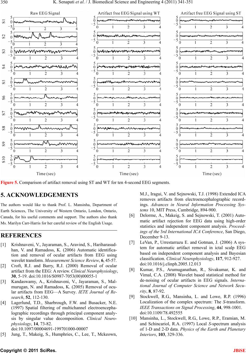

K. Senapati et al. / J. Biomedical Science and Engineering 4 (2011) 341-351 350
Figure 5. Comparison of artifact removal using ST and WT for ten 4-second EEG segments.
5. ACKNOWLEDGEMENTS
The authors would like to thank Prof. L. Mansinha, Department of
Earth Sciences, The University of Western Ontario, London, Ontario,
Canada, for his useful comments and support. The authors also thank
Ms. Marilyn Carr-Harris for her careful review of the English Usage.
REFERENCES
[1] Krishnaveni, V., Jayaraman, S., Aravind, S., Hariharasud-
han, V. and Ramadoss, K. (2006) Automatic identifica-
tion and removal of ocular artifacts from EEG using
wavelet transform. Measurement Science Review, 6, 45-57.
[2] Croft, R.J. and Barry, R.J. (2000) Removal of ocular
artifact from the EEG: A review. Clinical Neurophysiology,
30, 5-19. doi:10.1016/S0987-7053(00)00055-1
[3] Kandaswamy, A., Krishnaveni, V., Jayaraman, S., Mal-
murugan, N. and Ramadoss, K. (2005) Removal of ocu-
lar artifacts from EEG—A Survey. IETE Journal of Re-
search, 52, 112-130.
[4] Lagerlund, T.D., Sharbrough, F.W. and Busacker, N.E.
(1997) Spatial filtering of multichannel electroencepha-
lographic recordings through principal component analy-
sis by singular value decomposition. Clinical Neuro-
physiology, 14, 73-82.
doi:10.1097/00004691-199701000-00007
[5] Jung, T., Makeig, S., Humphries, C., Lee, T., Mckeown,
M.J., Iragui, V. and Sejnowski, T.J. (1998) Extended ICA
removes artifacts from electroencephalographic record-
ings. Advances in Neural Information Processing Sys-
tems 10, MIT Press, Cambridge, 894-900.
[6] Delorme, A., Makeig, S. and Sejnowski, T. (2001) Auto-
matic artifact rejection for EEG data using high-order
statistics and independent component analysis. Proceed-
ings of the 3rd International ICA Conference, San Diego,
December 9-13.
[7] LeV an, P., Urrestarrazu E. and Gotman, J. (2006) A sys-
tem for automatic artifact removal in ictal scalp EEG
based on independent component analysis and Bayesian
classification. Clinical Neurophysiology, 117 , 912-927.
doi:10.1016/j.clinph.2005.12.013
[8] Kumar, P.S., Arumuganathan, R., Sivakumar, K. and
Vimal, C.A. (2008) Wavelet based statistical method for
de-noising of ocular artifacts in EEG signals. Interna-
tional Journal of Computer Science and Network Secu-
rity, 8, 87-92.
[9] Stockwell, R.G., Mansinha, L. and Lowe, R.P. (1996)
Localization of the complex spectrum: The S-transform.
IEEE Transactions on Signal Processing, 44, 998-1001.
doi:10.1109/78.492555
[10] Mansinha, L., Stockwell, R.G., Lowe, R.P., Eramian, M.
and Schincariol, R.A. (1997) Local S-spectrum analysis
of 1-D and 2-D data. Physics of the Earth and Planetary
Interiors, 103, 329-336.
C
opyright © 2011 SciRes. JBiSE

K. Senapati et al. / J. Biomedical Science and Engineering 4 (2011) 341-351 351
doi:10.1016/S0031-9201(97)00047-2
[11] Moreau, E. and Macchi, O. (1993) New self adaptive
algorithms for source separation based on contrast func-
tions. Proceeding IEEE Signal Processing Workshop on
Higher Order Statistics, Lake Tahoe, June 1993, 215-219.
[12] Amari, S., Cichocki A. and Yang, H. (1996) A new
learning algorithm for blind signal separation. Advances
in Neural Information Processing, 8, 757-763.
[13] Amari, S. and Cichocki, A. (1998) Adaptive blind signal
processing-neural network approaches. Proceedings of
the IEEE, 86, 2026-2048. doi:10.1109/5.720251
[14] Hyvarinen, A. (1997) Independent component analysis
by minimization of mutual information (technical report).
Helsinki University of Technology, Helsinki.
[15] Lee, T.W., Girolami, M. and Sejnowski, T.J. (1999) In-
dependent component analysis using an extended info-
max algorithm for mix sub-gaussian and super-gaussian
sources. Neural Computation, 11, 417-441.
doi:10.1162/089976699300016719
[16] Cichicki, A. and Amari, S. (2002) Adaptive blind signal
and image processing: Learning algorithms and applica-
tions. John Wiley & Sons Ltd., New York.
doi:10.1002/0470845899
[17] Hyvärinen, A., Karhunen, J. and Oja, E. (2001) Inde-
pendent component analysis. John Wiley & Sons Ltd.,
New York.
[18] Bell, A. and Sejnowski, T. (1995) Information-maximi-
zation approach to blind separation and blind deconvolu-
tion. Neural Computation, 7, 1129-1159.
doi:10.1162/neco.1995.7.6.1129
[19] Daubechies. I. (1990) The wavelet transform, time-fre-
quency localization and signal analysis. IEEE Transac-
tions on Information Theory, 36, 961-1005.
doi:10.1109/18.57199
[20] Mallat, S. (1999) A wavelet tour of signal processing.
2nd Edition, Academic Press, San Diego.
[21] Rioul, O. and Vetterli, M. (1991) Wavelets and signal
processing. IEEE Signal Processing Magazine, 14-38.
[22] Chu, P.C. (1996) The S-transform for obtaining localized
spectra. Marine Technology Society Journal, 29, 28-38.
[23] Stockwell, R.G., Lowe, R.P. and Mansinha, L. (1996)
Localized cross spectral analysis with “phase corrected”
wavelets. The International Society for Optical Engi-
neering (SPIE) Proceedings 2762, Orlando, 8-12 April
1996, 557-564.
[24] Stockwell, R.G., Lowe, R.P. and Mansinha, L. (1997)
Instantaneous wavevector analysis. The International
Society for Optical Engineering (SPIE) Proceedings
3078, Orlando, 24 April 1997, 349-358.
[25] Stockwell, R.G. (1999) S-transform analysis of gravity
wave activity from a small scale network of airglow
imagers. Ph.D. Thesis, University of Western Ontario,
Ontario.
[26] Livanos, G., Ranganathan, N. and Jiang, J. (2000) Heart
sound analysis using the S-transform. IEEE Computers in
Cardiology, 27, 587-590.
[27] Varanini, M., De Paolis, G., Emdin, M., Macareta, A.,
Pola, S., Cipriani, M. and Marchesi, C. (1997) Spectral
analysis of cardiovascular time series by the S-transform.
IEEE Computers in Cardiology, 24, 383-386.
[28] Eramian, M.G., Schincariol, R.A., Mansinha, L. and
Stockwell, R.G. (1999) Generation of aquifer heterogene-
ity maps using two-dimensional spectral texture segmen-
tation techniques. Mathematical Geology, 31, 327-348.
doi:10.1023/A:1007578305616
[29] McFadden, P .D., Cook, J.G. and Forster, L.M. (1999)
Decomposition of gear vibration signals by the general-
ized S-transform. Mechanical Systems and Signal Proc-
essing, 13, 691-707. doi:10.1006/mssp.1999.1233
[30] Ventosa, S., Simon, C., Schimmel, M., Dañobeitia, J.J.
and Mànuel, A. (2008) The S-transform from a wavelet
point of view. IEEE Transactions on Signal Processing,
56, 2771-2780. doi:10.1109/TSP.2008.917029
[31] Stockwell, R.G. (2007) Why use the S-transform? AMS
Pseudo-differential operators: Partial differential equa-
tions and time-frequency analysis, 52, 279-309.
C
opyright © 2011 SciRes. JBiSE