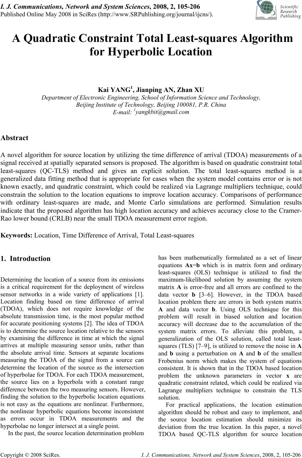I. J. Communications, Network and System Sciences, 2008, 2, 105-206
Published Online May 2008 in SciRes (http://www.SRPublishing.org/journal/ijcns/).
Copyright © 2008 SciRes. I. J. Communications, Network and System Sciences, 2008, 2, 105-206
A Quadratic Constraint Total Least-squares Algorithm
for Hyperbolic Location
Kai YANG1, Jianping AN, Zhan XU
Department of Electronic Engineering, School of Information Science and Technology,
Beijing Institute of Technology, Beijing 100081, P.R. China
Abstract
A novel algorithm for source location by utilizing the time difference of arrival (TDOA) measurements of a
signal received at spatially separated sensors is proposed. The algorithm is based on quadratic constraint total
least-squares (QC-TLS) method and gives an explicit solution. The total least-squares method is a
generalized data fitting method that is appropriate for cases when the system model contains error or is not
known exactly, and quadratic constraint, which could be realized via Lagrange multipliers technique, could
constrain the solution to the location equations to improve location accuracy. Comparisons of performance
with ordinary least-squares are made, and Monte Carlo simulations are performed. Simulation results
indicate that the proposed algorithm has high location accuracy and achieves accuracy close to the Cramer-
Rao lower bound (CRLB) near the small TDOA measurement error region.
Keywords: Location, Time Difference of Arrival, Total Least-squares
1. Introduction
Determining the location of a source from its emissions
is a critical requirement for the deployment of wireless
sensor networks in a wide variety of applications [1].
Location finding based on time difference of arrival
(TDOA), which does not require knowledge of the
absolute transmission time, is the most popular method
for accurate positioning systems [2]. The idea of TDOA
is to determine the source location relative to the sensors
by examining the difference in time at which the signal
arrives at multiple measuring sensor units, rather than
the absolute arrival time. Sensors at separate locations
measuring the TDOA of the signal from a source can
determine the location of the source as the intersection
of hyperbolae for TDOA. For each TDOA measurement,
the source lies on a hyperbola with a constant range
difference between the two measuring sensors. However,
finding the solution to the hyperbolic location equations
is not easy as the equations are nonlinear. Furthermore,
the nonlinear hyperbolic equations become inconsistent
as errors occur in TDOA measurements and the
hyperbolae no longer intersect at a single point.
In the past, the source location determination problem
has been mathematically formulated as a set of linear
equations Ax=b which is in matrix form and ordinary
least-squares (OLS) technique is utilized to find the
maximum-likelihood solution by assuming the system
matrix A is error-free and all errors are confined to the
data vector b [3–6]. However, in the TDOA based
location problem there are errors in both system matrix
A and data vector b. Using OLS technique for this
problem will result in biased solution and location
accuracy will decrease due to the accumulation of the
system matrix errors. To alleviate this problem, a
generalization of the OLS solution, called total least-
squares (TLS) [7–9], is utilized to remove the noise in A
and b using a perturbation on A and b of the smallest
Frobenius norm which makes the system of equations
consistent. It is shown that in the TDOA based location
problem the unknown parameters in vector x are
quadratic constraint related, which could be realized via
Lagrange multipliers technique to constrain the TLS
solution.
For practical applications, the location estimation
algorithm should be robust and easy to implement, and
the source location estimation should minimize its
deviation from the true location. In this paper, a novel
TDOA based QC-TLS algorithm for source location

A QUADRATIC CONSTRAINT TOTAL LEAST-SQUARES ALGORITHM 131
FOR HYPERBOLIC LOCATION
Copyright © 2008 SciRes. I. J. Communications, Network and System Sciences, 2008, 2, 105-206
problem is presented. The rest of the paper is organized
as follows. The formulation of TDOA based location
estimation problem is described in Section 2. In Section
3, this problem is shown to be in the form of an
overdetermined set of linear equations with errors in
both A and b and the QC-TLS algorithm is applied to
the TDOA measurement data for source location
estimation. Computer simulations are used to verify the
validity of the algorithm and simulation results are
presented in Section 4, which is followed by conclusions.
2. Problem Formulation
There are two basic ways to measure the TDOA in
wireless sensor networks: the direct way and the indirect
way. In the direct way, we could obtain the TDOA
through the use of cross-correlation techniques, in which
the received signal at one sensor is correlated with the
received signal at another sensor. The timing
requirement for this method is the synchronization of all
the receivers participating in the TDOA measurements,
which is more available in location applications.
However, in multipath channels there is ambiguity in
detecting the TDOA using cross-correlation techniques
since the correlation peak to be detected may not be
caused by the two direct line of sight (LOS) paths [10].
In the indirect way, we first obtain the arrival time of
received signal transmitted from the source at spatially
separated sensors and then subtract the measurements of
arrival time at two sensors to produce a relative TDOA.
TDOA also could be obtained by subtracting absolute
TOA measurements, but this requires the
synchronization of source and sensors. In this paper,
because of these factors above we obtain the TDOA by
subtracting the measurements of arrival time at two
sensors.
When TDOA based location method is adopted to
give source location estimation in wireless networks,
according to TDOA measurements a set of hyperbolic
equations is given by
()()
11 1
22
ss
,2,3,,
iii
ii i
rc rriM
rxx yy
τ
==−=
=−+−
L
(1)
where c is the speed of signal propagation, τi1 is the true
value of TDOA measurement between sensor i and 1, ri
is the distance between the source and sensor i, M is the
number of sensors, and (xs, ys) and (xi, yi) are the
coordinates of the source and sensor i respectively.
Solving those nonlinear equations is difficult.
Linearizing them and then solving is one possible way.
From (1), we have
11ii rrr+= (2)
Substituting the expressions of ri and r1 into (2) and
then squaring both sides of (2) produces
(
)
(
)
(
)( )
()()
()
1s11s1 11
22
2
111
1
2
iii
iii
x
xxxyyyyrr
xxyyr
−
−+−−+⋅
=−+−− (3)
Formulation it in matrix form we have
=
Axb (4)
where
[]
()()
()()
()()
212121
313131
111
111
22
2
212121
22
2
313131
22
2
111
1
2
MM M
T
ss
MMM
xxyyr
xxyyr
xxyyr
xxyyr
xxyy r
xxyy r
x
xyyr
−−
⎡⎤
⎢⎥
−−
⎢⎥
=⎢⎥
⎢⎥
−−
⎣⎦
=− −
⎡
⎤
−+−−
⎢
⎥
⎢
⎥
−+−−
=
⎢
⎥
⎢
⎥
⎢
⎥
−+−−
⎢
⎥
⎣
⎦
A
x
b
M
M
and the superscript T denotes the matrix transpose
operation.
In the absence of noise and interference, hyperbolae
from two or more sensors will intersect to determine a
unique location which means that the overdetermined set
of linear equations (4) is consistent. In the presence of
noise, more than two hyperbolae will not intersect at a
single point which means that (4) is inconsistent. In the
following section, we will develop the solution to the
overdetermined equations.
3. Hyperbolic Location Solution
In this section we first analyze the OLS solution to (4)
and then give the QC-TLS solution.
3.1. OLS Approach
In our applications, the usual assumption for OLS
approach is that the matrix A consists of M-1
observations on each of the 3 independent variables. The
dependent variable is represented by vector b, in which
we try keeping the correction term ∆b as small as
possible while simultaneously compensating for the
noise present in b by forcing Ax=b+∆b [7].
Under these assumptions the least-squares estimator
(
)
1
TT
−
=xAAAb
(5)

132 K. YANG ET AL.
Copyright © 2008 SciRes. I. J. Communications, Network and System Sciences, 2008, 2, 105-206
in which it is implicit that A is known exactly. Suppose
now that the elements of the A matrix contain errors.
The system matrix A resulting from the calculation of (4)
by using the measured values of TDOA can be given by
A=A0+E, where A0 and E represent the true value and
error respectively. Under the assumption that the error E
is reasonably small, retaining only the linear error terms,
the OLS estimator is given by [11]
()
()
(
)
11
0000 0
TTT T
−−
=+ −xEx AAEηAA AEx
(6)
where η is the vector of residuals b-Ax which would be
obtained if A were known accurately.
The sensitivity of each estimated parameter xk to each
element Aji of system matrix A comes immediately from
(6) by taking the derivative of xk with respect to Aji and
this yields
() ()
3
11
00 00
1
TT
k
jjli
ki kl
l
ji
x
A
x
A
η
−−
=
∂⎛⎞
=−
⎜⎟
∂⎝⎠
∑
AAAA (7)
The sensitivities are different, both in value and
ranking, from the sensitivities to change in the
dependent variable. It would in particular give details of
those observations most liable to cause estimation error.
3.2. QC-TLS Approach
In hyperbolic location problem, it can be argued that
both the system matrix A and vector b are subject to
error, which is out of accord with the assumption of
OLS. To
11
(, )ab
22
(, )ab
33
(, )ab
bxa=
a
b
Figure 1. Least-squares versus total least-squares
alleviate the effects of these errors, we propose to use
the TLS solution for the source location problem. The
total least-squares method [8,9], which is a natural
extension of LS when errors occur in all data, is devised
as a more global fitting technique than the ordinary
least-squares technique for solving overdetermined sets
of linear equations by trying to remove the data errors.
The LS and TLS measures of goodness are shown in
Figure 1. In the LS approach, it is the vertical distances
that are important; whereas in the TLS problem, it is the
perpendicular distances that are critical. So, from this
geometric interpretation, it’s shown that the TLS method
is better than the LS method with respect to the residual
error in the curve fitting.
When errors exist in TDOA measurements, (4) can be
represented by
(
)
00
+
=+AExbw
(8)
where E and w are the perturbations of A and b,
respectively. And (8) also can be put into the following
form
[][] ()
00
1
⎡⎤
−
+− =
⎢⎥
⎣⎦
bA wE0
x
MM (9a)
or
(
)
0=B+Dα0 (9b)
Where
[][]
000
,,1
T
T
⎡⎤
=−=− =
⎣⎦
BbADwEαx MM
The rank of matrix B0 is three, because it is equal to
the rank of matrix A0.
The TLS solution to this problem is to looks for the
minimal (in the Frobenius norm sense) perturbation
matrix E and perturbation vector w so that
{}
2
,,
ˆ,, argmin
F
=xEw xEwD (10)
subject to
(
)
00
+
=+AExbw
where the subscript F denotes the Frobenius norm.
The TLS optimization involves to find the optimum
ˆ α for α that minimizes the cost function
(
)
ˆ fα,
()
2
000
ˆˆˆˆ
TT
F
f==αBααBBα (11)
In practical applications, the value of matrix B0 is
unknown. We now make a singular value decomposition
(SVD) of the matrix B= [-b A], that is,
BB
H
B
=BUΣV (12)
where ΣB is composed of the singulars value of B. To
solve (11), matrix B0 can be replaced by a rank three
optimum approximation of B0, that is,
B3
H
B
=BUΣV
% (13)
where Σ3 is composed of the maximum three singulars
value of B. Now we have the cost function
(
)
ˆˆˆ
TT
f=ααBBα
%% (14)
The parameters in vector ˆ
α are subject to a quadratic
constraint

A QUADRATIC CONSTRAINT TOTAL LEAST-SQUARES ALGORITHM 133
FOR HYPERBOLIC LOCATION
Copyright © 2008 SciRes. I. J. Communications, Network and System Sciences, 2008, 2, 105-206
()()
22
2
1s1 s1
ˆˆˆ 110xxyyr+− +−−−=
(15)
or, equivalently, as
T
ˆˆ
10 −=αΣα (16)
where Σ=diag(1, 1, 1, −1) is a diagonal and orthonormal
matrix. The technique of Lagrange multipliers is used
and the modified cost function is of the form
(
)
{
}
()
ˆˆˆˆˆ 1
ˆˆ
TT T
TT
f λ
λ
λ
=+−
=+−
ααBBααΣα
αBB Σα
%%
%%
(17)
where λ is the Lagrange multiplier.
The required optimum parameter vector ˆ
α is found
by solving the following linear system of equations [12]
()
1
ˆ
Tk
λ +=BB Σα e
%% (18)
where, e1=[1 0 0 0] T , and normalizing constant k is
selected so that the first element of solution vector ˆ
α is
equal to one. Solving (18) is very easy, and it is
independent of normalization constant k, which is
unknown. Calculating the inverse of matrix
()
T
λ
+BB Σ
%%
and then normalizing the first element of ˆ
α, we can
obtain the solution vector. The QC-TLS solution vector
to (9) is
(
)
()
(
)
()
11
11
11
1111
ˆ
TT
TT TT
k
k
λλ
λλ
−−
−−
++
==
++
BB ΣeBBΣe
α
eBB ΣeeBBΣe
%% %%
%% %%
(19)
The estimated x and y coordinates of the source are
21
31
ˆ ˆ
ˆ ˆ
T
s
T
s
x
x
yy
=+
=+
αe
αe
(20)
where
[
]
[]
2
3
0100
0010
T
T
=
=
e
e
Lagrange Multiplier λ in the expression of solution
vector ˆ α is unknown. In order to find λ, we can impose
the quadratic constraint directly by substituting (19) into
(16), so that
()
()
()
()
11
11
11
1111
10
T
TT
TT TT
λλ
λλ
−−
−−
⎡⎤⎡⎤
++
⎢⎥⎢⎥
−=
⎢⎥⎢⎥
++
⎣⎦⎣⎦
BB ΣeBBΣe
Σ
eBBΣeeBBΣe
%% %%
%% %%
(21)
By using an eigenvalue factorization, the matrix
T
BBΣ
%% can be diagonalized as
1T−
=BBΣUΛU
%% (22)
where Λ=diag(γ1, γ2, γ3, γ4), γi, i=1, …, 4 are the
eigenvalues of the matrix T BBΣ
%% , and U is the
corresponding eigenmatrix of T BBΣ
%% . Substituting (22)
into (21) produces
(
)
()
1
21
1
2
11
11
10
T
T
λ
λ
−−
−−
+−=
⎡⎤
+
⎣⎦
eΣUΛIUe
eΣUΛIUe
(23)
For notational convenience, we define
[]
[]
[]
14
1234
1
12 3 4
1234
2
T
TTTT
3
iiiii
T
iiiii
pppp
qqqq
−
⎡
⎤
=
⎣
⎦
=
=
=
ΣU pppp
p
Uqqqq
q
(24)
Substituting (24) into (23), then the quadratic
constraint in the form of λ becomes
() ()()
()
4 42
11
2
11
2
4 4
11
11
0
ii
i
ii
i
ii
i
ii
i
pq
f
pq
λγλ
γλ
γλ
γλ
==
==
=⋅+
+
⎛⎞
−
⋅+=
⎜⎟
+
⎝⎠
∑∏
∑∏
(25)
Lagrange Multiplier λ can be solved from (25) by using
Newton’s method with zero as the initial guess.
To sum up, a brief description of the proposed TDOA
based location algorithm is as follows:
1) Calculate the optimum approximation of augmented
matrix B0 using (12) and (13).
2) Solve λ by finding the root of (25) using Newton’s
method.
3) Obtain the QC-TLS solution to (9) using (19) and
determine x and y coordinates of the source using
(20).
4. Simulations
We have proposed a QC-TLS algorithm for TDOA
based location problem. In this section, we evaluate its
performance at practical measurement error levels using
Monte-Carlo simulations.
Source and sensors were located in random positions
in a square of area 100×100 m2 as shown in Fig. 2. We
assumed that the TDOA measurement errors were white
random processes with zero mean and variance 2
TDOA
σ
,
and the TDOA variance of all sensor inputs were
identical. For simplicity, the TDOA variance was
translated into corresponding distance variance
σ2=(cσTDOA)2. Simulation results provided were averages
of 10000 independent runs. We compare the proposed
QC-TLS approach with OLS approach and CRLB.

134 K. YANG ET AL.
Copyright © 2008 SciRes. I. J. Communications, Network and System Sciences, 2008, 2, 105-206
Tables 1 and 2 compare the mean absolute location
errors (MALEs) of OLS and QC-TLS approach for
various TDOA error variances, and MALE was defined
as
()()
22
ˆˆ
ss ss
Exxyy
⎡⎤
−+−
⎢⎥
⎣⎦
. The number of
sensors was set to 7 and 10 for Table 1 and Table 2,
respectively. In Tables 1 and 2, CRLB, which is a
fundamental lower bound on the variance of any
unbiased estimator, is calculated using the functions in
[4]. The distance unit is meters. We observe that
increasing the number of sensors can increase the
location accuracy, because increasing the number of
sensors can provide more redundant information which
could be helpful for solving the overdetermined linear
equations.
-50 -40-30 -20 -1001020 3040 50
-50
-40
-30
-20
-10
0
10
20
30
40
50
X /m
Y /m
s e nsors
source
Figure 2. Location in 2-D plane
Table 1. comparison of MALEs for QC-TLS and OLS
method for various variances: seven sensors
σ2 0.1 0.01 0.001 0.0001
OLS 0.9359 0.2962 0.0939 0.0293
QC-TLS 0.7735 0.2236 0.0709 0.0221
CRLB 0.6706 0.2134 0.0677 0.0214
Table 2. comparison of MALEs for QC-TLS and OLS
method for various variances: ten sensors
σ2 0.1 0.01 0.001 0.0001
OLS 0.5801 0.1851 0.0571 0.0182
QC-TLS 0.5410 0.1501 0.0472 0.0150
CRLB 0.4280 0.1361 0.0428 0.0136
The performance of QC-TLS approach is much better
than OLS approach especially when the TDOA variance
is large, and it is closer to CRLB. They verify that the
proposed approach could inhibit the influence of TDOA
measurement errors on the estimation results better than
OLS. When TDOA variance is large, the noise in matrix
A, which would be alleviated by QC-TLS approach,
could significantly reduce the performance of OLS
approach.
Mean absolute location error is one of the metrics to
evaluate the performance of QC-TLS algorithm, and
computational complexity is another important metric to
evaluate the performance of algorithms. The price of the
better performance for QC-TLS is that its computational
complexity is larger than OLS. In the same simulation
condition, the time of 10000 independent runs for QC-
TLS and OLS are approximately 6153.6 ms and 1446.3
ms, respectively. It is obviously that QC-TLS algorithm
requires matrix singular value decomposition once,
eigenvalue decomposition once, Newton iteration once,
inverse operation once and matrix multiply operation
several times, whereas OLS algorithm only requires
matrix pseudoinverse operation once and matrix
multiply operation several times. It’s noteworthy that
QC-TLS algorithm performs better at a cost of larger
computational complexity.
5. Conclusions
A novel TDOA based quadratic constraint total least-
squares location algorithm is proposed in this paper. The
proposed algorithm utilizes TLS to inhibit the influence
of TDOA measurement errors. And the technique of
Lagrange multipliers is utilized to exploit the quadratic
constraint relation between the intermediate variables to
constrain the solution to the location equations and
improve the location accuracy. Simulation results
indicate that the proposed QC-TLS algorithm gives
better results than the OLS solution.
6. References
[1] N. Patwari, J. N. Ash, S. Kyperountas, A. O. Hero III, R.
L. Moses, and N. S. Correal, “Locating the Nodes:
Cooperative Localization in Wireless Sensor Networks,”
IEEE Signal Processing Magazine, vol. 22, no. 4, pp. 54–
68, July 2005.
[2] X. Jun, L. R. Ren, and J. D. Tan, “Research of TDOA
based self-localization approach in wireless sensor
network,” in proceedings of IEEE International
Conference on Intelligent Robots and Systems, Beijing,
pp. 2035–2040, October 2006.
[3] J. Smith and J. Abel, “Closed-form least-squares source
location estimation from range-difference
measurements,” IEEE Transactions on Acoustics, Speech,
and Signal Processing, vol. 35, pp. 1661–1669,
December 1987.
[4] Y. T. Chan and K. C. Ho, “A simple and efficient
estimation for hyperbolic location,” IEEE Transactions
on Signal processing, vol. 42, no. 8, pp. 1905–1915,
August 1994.
[5] R. Schmidt, “Least squares range difference location,”
IEEE Transactions on Aerospace and Electronic Systems,
vol. 32, no. 1, pp. 234–242, January 1996.
[6] Y. Huang, J. Benesty, G. W. Elko, and R. M. Mersereau,
“Real-time passive source localization: a practical linear-
correction least-squares approach,” IEEE Transactions

A QUADRATIC CONSTRAINT TOTAL LEAST-SQUARES ALGORITHM 135
FOR HYPERBOLIC LOCATION
Copyright © 2008 SciRes. I. J. Communications, Network and System Sciences, 2008, 2, 105-206
On Speech And Audio Processing, vol. 9, no. 8, pp. 943–
956, November 2001.
[7] T. J. Abatzoglou, J. M. Mendel, and G. A. Harada, “The
constrained total least squares technique and its
applications to harmonic superresolution,” IEEE
Transactions on Signal Processing, vol. 39, no. 5, pp.
1070–1087, May 1991.
[8] S. V. Huffel and J. Vandewalle, “The Total Least
Squares Problem: Computational Aspects and Analysis,”
Philadelphia: SIAM, 1991.
[9] I. Markovsky and S. V. Huffel, “Overview of total least-
squares methods,” Signal Processing, vol. 87 no. 10, pp.
2283–2302, October 2007.
[10] X. Li, “Super-Resolution TOA Estimation with Diversity
Techniques for Indoor Geolocation Applications,” Ph.D.
Dissertation, Worcester Polytechnic Institute, Worcester,
MA, 2003.
[11] S. D. Hodges and P. G. Moore, “Data Uncertainties and
Least Squares Regression,” Applied Statistics, vol. 21, pp.
185–195, 1972.
[12] J. A. Cadzow, “Spectral estimation: An overdetermined
rational model equation approach,” Proceedings of the
IEEE, vol. 70, no. 9, pp.907–939, September 1982.