ABSTRACT

Ultrahyperfunctions (UHF) are the generalization and extension to the complex plane of Schwartz’ tempered distributions. This effort is an application to Einstein’s gravity (EG) of the mathematical theory of convolution of Ultrahyperfunctions developed by Bollini et al. [1] [2] [3] [4]. A simplified version of these results was given in [5] and, based on them; a Quantum Field Theory (QFT) of EG [6] was obtained. Any kind of infinities is avoided by recourse to UHF. We will quantize EG by appealing to the most general quantization approach, the Schwinger-Feynman variational principle, which is more appropriate and rigorous that the popular functional integral method (FIM). FIM is not applicable here because our Lagrangian contains derivative couplings. We follow works by Suraj N. Gupta and Richard P. Feynman so as to undertake the construction of an EG-QFT. We explicitly use the Einstein Lagrangian as elaborated by Gupta [7], but choose a new constraint for the ensuing theory. In this way, we avoid the problem of lack of unitarity for the S matrix that afflicts the procedures of Gupta and Feynman. Simultaneously, we significantly simplify the handling of constraints, which eliminates the need to appeal to ghosts for guarantying unitarity of the theory. Our approach is obviously non-renormalizable. However, this inconvenience can be overcome by appealing to the mathematical theory developed by Bollini et al. [1] [2] [3] [4] [5]. Such developments were founded in the works of Alexander Grothendieck [8] and in the theory of Ultradistributions of Jose Sebastiao e Silva [9] (also known as Ultrahyperfunctions). Based on these works, an edifice has been constructed along two decades that are able to quantize non-renormalizable Field Theories (FT). Here we specialize this mathematical theory to discuss EG-QFT. Because we are using a Gupta-Feynman inspired EG Lagrangian, we are able to evade the intricacies of Yang-Mills theories.

Keywords:

Quantum Field Theory, Einstein Gravity, Non-Renormalizable Theories, Unitarity

1. Introduction

Quantifying Einstein gravity (EG) remains an open question, a kind of supreme desideratum for quantum field theory (QFT). The failure of some attempts in this direction is due to the fact that 1) they appeal to Rigged Hilber Space (RHS) with undefined metric, 2) problems of non-unitarity, and also 3) non-renormalizablity issues.

Here we build up a unitary EG’s QFT in the wake of related efforts by Suraj N. Gupta [7]. We deviate from his work by using a different EG-constraint, facing then a problem similar to that posed by Quantum Electrodynamics (QED). In order to quantize the concomitant non-renormalizable variational problem we appeal to mathematics developed by Bollini et al. [1] [2] [3] [4] [5], based upon the theory of Ultradistributions de J. Sebastiao e Silva (JSS) [9], also known as Ultrahyperfunctions (UHF). Any kind of infinities is avoided by recourse to UHF. The above cited mathematics was specifically devised to quantify non-renormalizable field theories. We consequently face a theory similar to QED, but endow with unitarity at all finite orders in power expansions in G (gravitation constant) of the EG Lagrangian. This was attempted without success first by Gupta and then by Feynman, in his Acta Physica Polonica work [10].

Mathematically, quantifying a non-renormalizable field theory is tantamount to suitably defining the product of two distributions (a product in a ring with zero-divisors in configuration space), an old problem in functional theory tackled successfully in [1] [2] [3] [4] [5].

Remarking that, in QFT, the problem of evaluating the product of distributions with coincident point singularities is related to the asymptotic behavior of loop integrals of propagators.

In references [1] [2] [3] [4], it was demonstrated that it is possible to define a general convolution between the ultradistributions of JSS [9] (Ultrahyperfunctions). This convolution yields another Ultrahyperfunction. Therefore, we have a product in a ring with zero divisors. Such a ring is the space of distributions of exponential type, or ultradistributions of exponential type obtained applying the anti-Fourier transform to the space of tempered ultradistributions or ultradistributions of exponential type.

We must clarify at this point that the ultrahyperfunctions, our present protagonists, are the generalization and extension to the complex plane of the Schwartz tempered distributions and the distributions of exponential type. That is the tempered distributions and those of exponential type are a subset of the ultrahyprefunctions.

In our work we do not use counter-terms to get rid of infinities, because our convolutions are always finite. We do not want counter-terms, since a non-renormalizable theory involves an infinite number of them.

At the same time, we conserve all extant solutions to the problem of running coupling constants and the renormalization group. The convolution, once obtained, converts configuration space into a ring with zero-divisors. In it, one has now defined a product between the ring-elements. Thus, any unitary-causal-Lorentz invariant theory quantified in such a manner becomes predictive. The distinction between renormalizable on non-renormalizable QFT’s becomes unnecessary now.

With our convolution, that uses Laurent’s expansions (LE) in the parameter employed to define the LE, all finite constants of the convolutions become completely determined, eliminating arbitrary choices of finite constants. This is tantamount to eliminating all finite renormalizations of the theory. The independent term in the Laurent expansion yield the convolution value. This translates to configuration space the product-operation in a ring with divisors of zero.

We have already obtained an EG-OFT in [6] by recourse to the mathematics elaborated in [5]. What we do here is an extended EG-QFT, using the more general mathematical approach of [3].

The manuscript is organized as follows:

• Section 2 presents preliminary materials.

• In Section 3 we introduce the convolution of Ultrahyperfunctions, our present protagonists.

• Section 4 is devoted to the QFT Lagrangian for EG.

• In Section 5 we quantize the ensuing theory.

• In Section 6 the graviton’s self-energy is evaluated up to second order.

• In Section 7 we introduce axions into our picture and deal with the axions gravitons interaction.

• In Section 8 we calculate the graviton’s self-energy in the presence of axions.

• In Section 9 we evaluate, up to second order, the axion’s self-energy.

• Finally, in Section 10, some conclusions are drawn.

2. Preliminary Materials

We do not deal in this effort with the popular functional integral method (FIM). Instead, we appeal here to the most general quantification approach, Schwinger-Feynman variational principle [11], which is able to deal even with high order supersymmetric theories, as exemplified by [12] [13]. Such theories cannot be quantized with the usual Dirac-brackets technique.

We introduce the action for a set of fields defined by

$\mathcal{S}\left[\sigma \left(x\right)\mathrm{,}{\sigma }_0\mathrm{,}{\varphi }_A\left(x\right)\right]={\displaystyle \underset{{\sigma }_0}{\overset{\sigma \left(x\right)}{\int }}}\mathcal{L}\left[{\varphi }_A\left(\xi \right)\mathrm{,}{\partial }_{\mu }{\varphi }_A\left(\xi \right)\mathrm{,}\xi \right]\text{d}\xi \mathrm{,}$ (2.1)

where $\sigma \left(x\right)$ if a space-like surface passing through the point x. ${\sigma }_0$ is that surface at the remote past, at which all field variations vanish. The Schwinger-Feynman variational principle dictates that:

“Any Hermitian infinitesimal variation $\delta \mathcal{S}$ of the action induces a canonical transformation of the vector space in which the quantum system is defined, and the generator of this transformation is this same operator $\delta \mathcal{S}$ ”.

Accordingly, the following equality holds:

$\delta {\varphi }_A=i\left[\delta \mathcal{S}\mathrm{,}{\varphi }_A\right]\mathrm{.}$ (2.2)

Thus, for a Poincare transformation we have

$\delta \mathcal{S}=a^{\mu }{\mathcal{P}}_{\mu }+\frac{1}{2}{a}^{\mu v}{\mathcal{M}}_{\mu v}\mathrm{,}$ (2.3)

where the field variation is given by

$\delta {\varphi }_a=a^{\mu }{\hat{P}}_{\mu }{\varphi }_A+\frac{1}{2}{a}^{\mu v}{\hat{M}}_{\mu v}{\varphi }_A\mathrm{.}$ (2.4)

From (2.2) one gathers that

${\partial }_{\mu }{\varphi }_A=i\left[{\mathcal{P}}_{\mu }\mathrm{,}{\varphi }_A\right]\mathrm{.}$ (2.5)

Specifically,

${\partial }_0{\varphi }_A=i\left[{\mathcal{P}}_0\mathrm{,}{\varphi }_A\right]\mathrm{.}$ (2.6)

This last result will be employed in quantizing EG.

3. The Convolution of Two Lorentz Invariant Tempered Ultradistributions

In [3] we have obtained a conceptually simple but rather lengthy expression for the convolution of two Lorentz invariant tempered ultradistributions:

$\begin{array}{l}{H}_{\lambda }\left(\rho \mathrm{,}\Lambda \right)\\ =\frac{1}{8{\pi }^2\rho }{\displaystyle \underset{{\Gamma }_1}{\int }}{\displaystyle \underset{{\Gamma }_2}{\int }}F\left({\rho }_1\right)G\left({\rho }_2\right){\rho }_1^{\lambda }{\rho }_2^{\lambda }\{\Theta \left[\Im \left(\rho \right)\right]\{\left[ln\left(-{\rho }_1+\Lambda \right)-ln\left(-{\rho }_1-\Lambda \right)\right]\underset{}{\overset{}{\underset{}{\underset{}{}}}}\\ \times \left[ln\left(-{\rho }_2+\Lambda \right)-ln\left(-{\rho }_2-\Lambda \right)\right]\sqrt{4\left({\rho }_1+\Lambda \right)\left({\rho }_2+\Lambda \right)-{\left(\rho -{\rho }_1-{\rho }_2-2\Lambda \right)}^2}\\ \times ln\left[\frac{\sqrt{4\left({\rho }_1+\Lambda \right)\left({\rho }_2+\Lambda \right)-{\left(\rho -{\rho }_1-{\rho }_2-2\Lambda \right)}^2}-i\left(\rho -{\rho }_1-{\rho }_2-2\Lambda \right)}{2\sqrt{\left({\rho }_1+\Lambda \right)\left({\rho }_2+\Lambda \right)}}\right]\\ +\left[ln\left({\rho }_1+\Lambda \right)-ln\left({\rho }_1-\Lambda \right)\right]\left[ln\left({\rho }_2+\Lambda \right)-ln\left({\rho }_2-\Lambda \right)\right]\end{array}$

$\begin{array}{l}\times \sqrt{4\left({\rho }_1-\Lambda \right)\left({\rho }_2-\Lambda \right)-{\left(\rho -{\rho }_1-{\rho }_2+2\Lambda \right)}^2}\\ \times ln\left[\frac{\sqrt{4\left({\rho }_1-\Lambda \right)\left({\rho }_2-\Lambda \right)-{\left(\rho -{\rho }_1-{\rho }_2+2\Lambda \right)}^2}-i\left(\rho -{\rho }_1-{\rho }_2+2\Lambda \right)}{2\sqrt{\left({\rho }_1-\Lambda \right)\left({\rho }_2-\Lambda \right)}}\right]\\ +\left[ln\left({\rho }_1+\Lambda \right)-ln\left({\rho }_1-\Lambda \right)\right]\left[ln\left(-{\rho }_2+\Lambda \right)-ln\left(-{\rho }_2-\Lambda \right)\right]\end{array}$

$\begin{array}{l}\times \{\frac{i\pi }{2}\left[\sqrt{4\left({\rho }_1+\Lambda \right)\left({\rho }_2-\Lambda \right)-{\left(\rho -{\rho }_1-{\rho }_2\right)}^2}-i\left(\rho -{\rho }_1-{\rho }_2\right)\right]\underset{}{\overset{}{\underset{}{\underset{}{}}}}\\ +\sqrt{4\left({\rho }_1+\Lambda \right)\left({\rho }_2-\Lambda \right)-{\left(\rho -{\rho }_1-{\rho }_2\right)}^2}\end{array}$

$\begin{array}{l}\times ln\left[\frac{\sqrt{4\left({\rho }_1+\Lambda \right)\left({\rho }_2-\Lambda \right)-{\left(\rho -{\rho }_1-{\rho }_2\right)}^2}-i\left(\rho -{\rho }_1-{\rho }_2\right)}{2i\sqrt{-\left({\rho }_1+\Lambda \right)\left({\rho }_2-\Lambda \right)}}\right]\}\\ +\left[ln\left(-{\rho }_1+\Lambda \right)-ln\left(-{\rho }_1-\Lambda \right)\right]\left[ln\left({\rho }_2+\Lambda \right)-ln\left({\rho }_2-\Lambda \right)\right]\\ \times \{\frac{i\pi }{2}\left[\sqrt{4\left({\rho }_1-\Lambda \right)\left({\rho }_2+\Lambda \right)-{\left(\rho -{\rho }_1-{\rho }_2\right)}^2}-i\left(\rho -{\rho }_1-{\rho }_2\right)\right]\underset{}{\overset{}{\underset{}{\underset{}{}}}}\\ +\sqrt{4\left({\rho }_1-\Lambda \right)\left({\rho }_2+\Lambda \right)-{\left(\rho -{\rho }_1-{\rho }_2\right)}^2}\\ \times ln\left[\frac{\sqrt{4\left({\rho }_1-\Lambda \right)\left({\rho }_2+\Lambda \right)-{\left(\rho -{\rho }_1-{\rho }_2\right)}^2}-i\left(\rho -{\rho }_1-{\rho }_2\right)}{2i\sqrt{-\left({\rho }_1-\Lambda \right)\left({\rho }_2+\Lambda \right)}}\right]\}\}\end{array}$

$\begin{array}{l}-\Theta \left[-\Im \left(\rho \right)\right]\{\left[ln\left(-{\rho }_1+\Lambda \right)-ln\left(-{\rho }_1-\Lambda \right)\right]\left[ln\left(-{\rho }_2+\Lambda \right)-ln\left(-{\rho }_2-\Lambda \right)\right]\underset{}{\overset{}{\underset{}{\underset{}{}}}}\\ \times \sqrt{4\left({\rho }_1-\Lambda \right)\left({\rho }_2-\Lambda \right)-{\left(\rho -{\rho }_1-{\rho }_2+2\Lambda \right)}^2}\\ \times ln\left[\frac{\sqrt{4\left({\rho }_1-\Lambda \right)\left({\rho }_2-\Lambda \right)-{\left(\rho -{\rho }_1-{\rho }_2+2\Lambda \right)}^2}-i\left(\rho -{\rho }_1-{\rho }_2+2\Lambda \right)}{2\sqrt{\left({\rho }_1-\Lambda \right)\left({\rho }_2-\Lambda \right)}}\right]\\ +\left[ln\left({\rho }_1+\Lambda \right)-ln\left({\rho }_1-\Lambda \right)\right]\left[ln\left({\rho }_2+\Lambda \right)-ln\left({\rho }_2-\Lambda \right)\right]\\ \times \sqrt{4\left({\rho }_1+\Lambda \right)\left({\rho }_2+\Lambda \right)-{\left(\rho -{\rho }_1-{\rho }_2-2\Lambda \right)}^2}\end{array}$

$\begin{array}{l}\times ln\left[\frac{\sqrt{4\left({\rho }_1+\Lambda \right)\left({\rho }_2+\Lambda \right)-{\left(\rho -{\rho }_1-{\rho }_2-2\Lambda \right)}^2}-i\left(\rho -{\rho }_1-{\rho }_2-2\Lambda \right)}{2\sqrt{\left({\rho }_1+\Lambda \right)\left({\rho }_2+\Lambda \right)}}\right]\\ +\left[ln\left({\rho }_1+\Lambda \right)-ln\left({\rho }_1-\Lambda \right)\right]\left[ln\left(-{\rho }_2+\Lambda \right)-ln\left(-{\rho }_2-\Lambda \right)\right]\\ \times \{\frac{i\pi }{2}\left[\sqrt{4\left({\rho }_1-\Lambda \right)\left({\rho }_2+\Lambda \right)-{\left(\rho -{\rho }_1-{\rho }_2\right)}^2}-i\left(\rho -{\rho }_1-{\rho }_2\right)\right]\underset{}{\overset{}{\underset{}{\underset{}{}}}}\\ +\sqrt{4\left({\rho }_1-\Lambda \right)\left({\rho }_2+\Lambda \right)-{\left(\rho -{\rho }_1-{\rho }_2\right)}^2}\\ \times ln\left[\frac{\sqrt{4\left({\rho }_1-\Lambda \right)\left({\rho }_2+\Lambda \right)-{\left(\rho -{\rho }_1-{\rho }_2\right)}^2}-i\left(\rho -{\rho }_1-{\rho }_2\right)}{2i\sqrt{-\left({\rho }_1-\Lambda \right)\left({\rho }_2+\Lambda \right)}}\right]\}\end{array}$

$\begin{array}{l}+\left[ln\left(-{\rho }_1+\Lambda \right)-ln\left(-{\rho }_1-\Lambda \right)\right]\left[ln\left({\rho }_2+\Lambda \right)-ln\left({\rho }_2-\Lambda \right)\right]\\ \times \{\frac{i\pi }{2}\left[\sqrt{4\left({\rho }_1+\Lambda \right)\left({\rho }_2-\Lambda \right)-{\left(\rho -{\rho }_1-{\rho }_2\right)}^2}-i\left(\rho -{\rho }_1-{\rho }_2\right)\right]\underset{}{\overset{}{\underset{}{\underset{}{}}}}\\ +\sqrt{4\left({\rho }_1+\Lambda \right)\left({\rho }_2-\Lambda \right)-{\left(\rho -{\rho }_1-{\rho }_2\right)}^2}\end{array}$

$\begin{array}{l}\times ln\left[\frac{\sqrt{4\left({\rho }_1+\Lambda \right)\left({\rho }_2-\Lambda \right)-{\left(\rho -{\rho }_1-{\rho }_2\right)}^2}-i\left(\rho -{\rho }_1-{\rho }_2\right)}{2i\sqrt{-\left({\rho }_1+\Lambda \right)\left({\rho }_2-\Lambda \right)}}\right]\}\}\\ -\frac{i}{2}\{\left[ln\left(-{\rho }_1+\Lambda \right)-ln\left(-{\rho }_1-\Lambda \right)\right]\left[ln\left(-{\rho }_2+\Lambda \right)-ln\left(-{\rho }_2-\Lambda \right)\right]\end{array}$

$\begin{array}{l}\times \left({\rho }_1-{\rho }_2\right)\left[ln\left(i\sqrt{\frac{{\rho }_1+\Lambda }{{\rho }_2+\Lambda }}\right)+ln\left(-i\sqrt{\frac{{\rho }_1-\Lambda }{{\rho }_2-\Lambda }}\right)\right]\\ +\left[ln\left({\rho }_1+\Lambda \right)-ln\left({\rho }_1-\Lambda \right)\right]\left[ln\left({\rho }_2+\Lambda \right)-ln\left({\rho }_2-\Lambda \right)\right]\\ \times \left({\rho }_1-{\rho }_2\right)\left[ln\left(-i\sqrt{\frac{\Lambda -{\rho }_1}{\Lambda -{\rho }_2}}\right)+ln\left(i\sqrt{\frac{\Lambda +{\rho }_1}{\Lambda +{\rho }_2}}\right)\right]\\ +\left[ln\left({\rho }_1+\Lambda \right)-ln\left({\rho }_1-\Lambda \right)\right]\left[ln\left(-{\rho }_2+\Lambda \right)-ln\left(-{\rho }_2-\Lambda \right)\right]\\ \times \{\left({\rho }_1-{\rho }_2\right)\left[ln\left(\sqrt{\frac{\Lambda +{\rho }_1}{\Lambda -{\rho }_2}}\right)+ln\left(\sqrt{\frac{\Lambda -{\rho }_1}{\Lambda +{\rho }_2}}\right)\right]\end{array}$

$\begin{array}{l}+\frac{{\rho }_1-{\rho }_2}{2}[ln\left(-{\rho }_1-{\rho }_2+\Lambda \right)-ln\left(-{\rho }_1-{\rho }_2-\Lambda \right)\\ -ln\left({\rho }_1+{\rho }_2+\Lambda \right)+ln\left({\rho }_1+{\rho }_2-\Lambda \right)]+{\rho }_2[ln\left(-{\rho }_1-{\rho }_2+\Lambda \right)\\ \underset{}{\underset{}{}}-ln\left(-{\rho }_1-{\rho }_2-\Lambda \right)]+{\rho }_1\left[ln\left({\rho }_1+{\rho }_2+\Lambda \right)-ln\left({\rho }_1+{\rho }_2-\Lambda \right)\right]\}\\ \left[ln\left(-{\rho }_1+\Lambda \right)-ln\left(-{\rho }_1-\Lambda \right)\right]\left[ln\left({\rho }_2+\Lambda \right)-ln\left({\rho }_2-\Lambda \right)\right]\\ \times \{\left({\rho }_1-{\rho }_2\right)\left[ln\left(\sqrt{\frac{\Lambda -{\rho }_1}{\Lambda +{\rho }_2}}\right)+ln\left(\sqrt{\frac{\Lambda +{\rho }_1}{\Lambda -{\rho }_2}}\right)\right]\underset{}{\overset{}{\underset{}{\underset{}{}}}}\end{array}$

$\begin{array}{l}+\frac{{\rho }_1-{\rho }_2}{2}[ln\left({\rho }_1+{\rho }_2+\Lambda \right)-ln\left({\rho }_1+{\rho }_2-\Lambda \right)\\ -ln\left(-{\rho }_1-{\rho }_2+\Lambda \right)+ln\left(-{\rho }_1-{\rho }_2-\Lambda \right)]+{\rho }_1[ln\left(-{\rho }_1-{\rho }_2+\Lambda \right)\\ \underset{}{\overset{}{\underset{}{}}}-ln\left(-{\rho }_1-{\rho }_2-\Lambda \right)]+{\rho }_2\left[ln\left({\rho }_1+{\rho }_2+\Lambda \right)-ln\left({\rho }_1+{\rho }_2-\Lambda \right)\right]\}\}\}\text{d}{\rho }_1\text{d}{\rho }_2\end{array}$ (3.1)

This defines an ultradistribution in the variables $\rho$ and $\Lambda$ for

$\left|\Im \left(\rho \right)\right|>\Im \left(\Lambda \right)>\left|\Im \left({\rho }_1\right)\right|+\left|\Im \left({\rho }_2\right)\right|$

Let $\mathfrak{B}$ be a vertical band contained in the complex $\lambda$ -plane $\mathfrak{P}$. Integral (3.1) is an analytic function of $\lambda$ defined in the domain $\mathfrak{B}$. Moreover, it is bounded by a power of $\left|\rho \Lambda \right|$. Then, $H_{\lambda }\left(\rho \mathrm{,}\Lambda \right)$ can be analytically continued to other parts of $\mathfrak{P}$. Thus, we define

$H\left(\rho \right)=H^{\left(0\right)}\left(\rho \mathrm{,}i{0}^{+}\right)$ (3.2)

$H_{\lambda }\left(\rho \mathrm{,}i{0}^{+}\right)={\displaystyle \underset{-m}{\overset{\infty }{\sum }}}{H}^{\left(n\right)}\left(\rho \mathrm{,}i{0}^{+}\right){\lambda }^n$ (3.3)

As in the other cases, we define now

$\left\{F\ast G\right\}\left(\rho \right)=H\left(\rho \right)$ (3.4)

as the convolution of two Lorentz invariant tempered ultradistributions.

The Feynman propagators corresponding to a massless particle F and a massive particle G are, respectively, the following ultrahyperfunctions:

$F\left(\rho \right)=-\Theta \left[-\Im \left(\rho \right)\right]{\rho }^{-1}$

$G\left(\rho \right)=-\Theta \left[-\Im \left(\rho \right)\right]{\left(\rho +m^2\right)}^{-1}$ (3.5)

where $\rho$ is the complex variable, such that on the real axis one has $\rho =k_1^2+k_2^2+k_3^2-k_0^2$. For them, the following equalities are satisfied

${\rho }^{\lambda }F\left(\rho \right)=-\Theta \left[-\Im \left(\rho \right)\right]{\rho }^{\lambda -1}$

${\rho }^{\lambda }G\left(\rho \right)=-\Theta \left[-\Im \left(\rho \right)\right]{\left(\rho +m^2\right)}^{\lambda -1}$ (3.6)

where we have used: ${\left(\rho +m^2\right)}^{\lambda }\simeq {\rho }^{\lambda }$, since we have chosen m to be very small. On the real axis, the previously defined propagators are given by:

$f\left(\rho \right)=F\left(\rho +i0\right)-F\left(\rho -i0\right)={\left(\rho -i0\right)}^{-1}$

$g\left(\rho \right)=G\left(\rho +i0\right)-G\left(\rho -i0\right)={\left(\rho +m^2-i0\right)}^{-1}$ (3.7)

These are the usual expressions for Feynman propagators.

Consider first the convolution of two massless propagators. We use (3.6), since here the corresponding ultrahyperfunctions do not have singularities in the complex plane. We obtain from (3.1) a simplified expression for the convolution:

$h_{\lambda }\left(\rho \right)=\frac{\pi }{2\rho }\underset{-\infty }{\overset{\infty }{{\displaystyle \int \int }}}{\left({\rho }_1-i0\right)}^{\lambda -1}{\left({\rho }_2-i0\right)}^{\lambda -1}{\left[{\left(\rho -{\rho }_1-{\rho }_2\right)}^2-4{\rho }_1{\rho }_2\right]}_{+}^{\frac{1}{2}}\text{d}{\rho }_1\text{d}{\rho }_2$ (3.8)

This expression is nothing other than the usual convolution:

$h_{\lambda }\left(\rho \right)={\left(\rho -i0\right)}^{\lambda -1}\ast {\left(\rho -i0\right)}^{\lambda -1}$ (3.9)

In the same way, we obtain for massive propagators:

$h_{\lambda }\left(\rho \right)={\left(\rho +m^2-i0\right)}^{\lambda -1}\ast {\left(\rho -m^2-i0\right)}^{\lambda -1}$ (3.10)

These last two expressions are the ones we will use later to evaluate the graviton’s self-energy.

4. The Lagrangian of Einstein’s QFT

Our EG Lagrangian reads [7]

${\mathcal{L}}_G=\frac{1}{{\kappa }^2}R\sqrt{\left|g\right|}-\frac{1}{2}{\eta }_{\mu v}{\partial }_{\alpha }{h}^{\mu \alpha }{\partial }_{\beta }{h}^{v\beta }\mathrm{,}$ (4.1)

where ${\eta }^{\mu \nu }=diag\left(\mathrm{1,1,1,}-1\right)$,$h^{\mu \nu }=\sqrt{\left|g\right|}{g}^{\mu \nu }$ The second term in (4.1) fixes the gauge. We effect now the linear approximation

$h^{\mu v}={\eta }^{\mu v}+\kappa {\varphi }^{\mu v}\mathrm{,}$ (4.2)

where ${\kappa }^2$ is the gravitation’s constant and ${\varphi }^{\mu v}$ the graviton field. We write

${\mathcal{L}}_G={\mathcal{L}}_L+{\mathcal{L}}_I\mathrm{,}$ (4.3)

where

${\mathcal{L}}_L=-\frac{1}{4}\left[{\partial }_{\lambda }{\varphi }_{\mu v}{\partial }^{\lambda }{\varphi }^{\mu v}-2{\partial }_{\alpha }{\varphi }_{\mu \beta }{\partial }^{\beta }{\varphi }^{\mu \alpha }+2{\partial }^{\alpha }{\varphi }_{\mu \alpha }{\partial }_{\beta }{\varphi }^{\mu \beta }\right]\mathrm{,}$ (4.4)

and, up to 2nd order, one has [7]:

${\mathcal{L}}_I=-\frac{1}{2}\kappa {\varphi }^{\mu v}\left[\frac{1}{2}{\partial }_{\mu }{\varphi }^{\lambda \rho }{\partial }_v{\varphi }_{\lambda \rho }+{\partial }_{\lambda }{\varphi }_{\mu \beta }{\partial }^{\beta }{\varphi }_v^{\lambda }-{\partial }_{\lambda }{\varphi }_{\mu \rho }{\partial }^{\lambda }{\varphi }_v^{\rho }\right]\mathrm{,}$ (4.5)

having made use of the constraint

${\varphi }_{\mu }^{\mu }=0.$ (4.6)

This constraint is required in order to satisfy gauge invariance [14] For the graviton we have then

$\square {\varphi }_{\mu v}=\mathrm{0,}$ (4.7)

whose solution is

${\varphi }_{\mu v}=\frac{1}{{\left(2\pi \right)}^{\frac{3}{2}}}{\displaystyle \int }\left[\frac{a_{\mu v}\left(k\right)}{\sqrt{2k_0}}{\text{e}}^{i{k}_{\mu }{x}^{\mu }}+\frac{a_{\mu v}^{+}\left(k\right)}{\sqrt{2k_0}}{\text{e}}^{-i{k}_{\mu }{x}^{\mu }}\right]{\text{d}}^{3}k\mathrm{,}$ (4.8)

with $k_0=\left|k\right|$.

5. Quantization of the Theory

We need some definitions. The energy-momentum tensor reads

$T_{\rho }^{\lambda }=\frac{\partial \mathcal{L}}{\partial {\partial }^{\rho }{\varphi }^{\mu v}}{\partial }^{\lambda }{\varphi }^{\mu v}-{\delta }_{\rho }^{\lambda }\mathcal{L}\mathrm{,}$ (5.1)

and the time-component of the four-momentum is

${\mathcal{P}}_0={\displaystyle \int }{T}_0^0{\text{d}}^{3}x\mathrm{.}$ (5.2)

Using (4.4) we have

$\begin{array}{c}{T}_0^0=\frac{1}{4}[{\partial }_0{\varphi }_{\mu v}{\partial }^0{\varphi }^{\mu v}+{\partial }_j{\varphi }_{\mu v}{\partial }^j{\varphi }^{\mu v}-2{\partial }_{\alpha }{\varphi }_{\mu 0}{\partial }^0{\varphi }^{\mu \alpha }-2{\partial }_{\alpha }{\varphi }_{\mu j}{\partial }^j{\varphi }^{\mu \alpha }\\ +2{\partial }_{\alpha }{\varphi }^{\mu \alpha }{\partial }_0{\varphi }_{\mu }^0+2{\partial }_{\alpha }{\varphi }^{\mu \alpha }{\partial }_j{\varphi }_{\mu }^j]\mathrm{.}\end{array}$ (5.3)

Consequently,

${\mathcal{P}}_0=\frac{1}{4}{\displaystyle \int }\left|k\right|\left[a_{\mu v}\left(k\right)a^{+\mu v}\left(k\right)+a^{+\mu v}\left(k\right)a_{\mu v}\left(k\right)\right]{\text{d}}^{3}k\mathrm{.}$ (5.4)

Appeal to (2.6) leads to

$\left[{\mathcal{P}}_0\mathrm{,}{a}_{\mu v}\left(k\right)\right]=-k_0{a}_{\mu v}(k)$

$\left[{\mathcal{P}}_0\mathrm{,}{a}^{+\mu v}\left(k\right)\right]=k_0{a}^{+\mu v}\left(k\right)\mathrm{.}$ (5.5)

From the last relation in (5.5) one gathers that

$\left|k\right|a^{+\rho \lambda }\left(k^{\prime }\right)=\frac{1}{2}{\displaystyle \int }\left|\stackrel{\to }{k}\right|\left[a_{\mu v}\left(k\right)\mathrm{,}{a}^{+\rho \lambda }\left(k^{\prime }\right)\right]a^{+\mu v}\left(k\right){\text{d}}^{3}k\mathrm{.}$ (5.6)

The solution of this integral equation is

$\left[a_{\mu v}\left(k\right)\mathrm{,}{a}^{+\rho \lambda }\left(k^{\prime }\right)\right]=\left[{\delta }_{\mu }^{\rho }{\delta }_v^{\lambda }+{\delta }_v^{\rho }{\delta }_{\mu }^{\lambda }\right]\delta \left(k-k^{\prime }\right)\mathrm{.}$ (5.7)

As customary, the physical state $|\psi \rangle$ of the theory is defined via the equation

${\varphi }_{\mu }^{\mu }|\psi \rangle =0.$ (5.8)

We use now the usual definition

${\Delta }_{\mu \nu }^{\rho \lambda }\left(x-y\right)=\langle 0|T\left[{\varphi }_{\mu \nu }\left(x\right){\varphi }^{\rho \lambda }\left(y\right)\right]|0\rangle \mathrm{.}$ (5.9)

The graviton’s propagator then turns out to be

${\Delta }_{\mu \nu }^{\rho \lambda }\left(x-y\right)=\frac{i}{{\left(2\pi \right)}^4}\left({\delta }_{\mu }^{\rho }{\delta }_v^{\lambda }+{\delta }_v^{\rho }{\delta }_{\mu }^{\lambda }\right){\displaystyle \int }\frac{{\text{e}}^{i{k}_{\mu }\left(x^{\mu }-y^{\mu }\right)}}{k^2-i0}{\text{d}}^{4}k\mathrm{.}$ (5.10)

As a consequence, we can write

${\mathcal{P}}_0=\frac{1}{4}{\displaystyle \int }\left|k\right|\left[a_{\mu v}\left(k\right)a^{+\mu v}\left(k^{\prime }\right)+a^{+\mu v}\left(k^{\prime }\right)a_{\mu v}\left(k\right)\right]\delta \left(k-k^{\prime }\right){\text{d}}^{3}k{\text{d}}^3{k}^{\prime }\mathrm{,}$ (5.11)

or

${\mathcal{P}}_0=\frac{1}{4}{\displaystyle \int }\left|k\right|\left[2a^{+\mu v}\left(k^{\prime }\right)a_{\mu v}\left(k\right)+\delta \left(k-k^{\prime }\right)\right]\delta \left(k-k^{\prime }\right){\text{d}}^{3}k{\text{d}}^3{k}^{\prime }\mathrm{.}$ (5.12)

Thus, we obtain

${\mathcal{P}}_0=\frac{1}{2}{\displaystyle \int }\left|k\right|a^{+\mu v}\left(k\right)a_{\mu v}\left(k\right){\text{d}}^{3}k\mathrm{,}$ (5.13)

where we have used the fact that the product of two deltas with the same argument vanishes [1], i.e., $\delta \left(k-k^{\prime }\right)\delta \left(k-k^{\prime }\right)=0$. This illustrates the fact that using Ultrahyperfunctions is here equivalent to adopting the normal order in the definition of the time-component of the four-momentum

${\mathcal{P}}_0=\frac{1}{4}{\displaystyle \int }\left|k\right|\mathrm{<mo>\; :\; </mo>}\left[a_{\mu v}\left(k\right)a^{+\mu v}\left(k\right)+a^{+\mu v}\left(k\right)a_{\mu v}\left(k\right)\right]\mathrm{<mo>\; :\; </mo>}{\text{d}}^{3}k\mathrm{.}$ (5.14)

Now, we must insist on the fact that the physical state should satisfy not only Equation (5.8) but also the relation (see [7])

${\partial }_{\mu }{\varphi }^{\mu v}|\psi \rangle =0.$ (5.15)

The ensuing theory is similar to the QED-one obtained via the quantization approach of Gupta-Bleuler. This implies that the theory is unitary for any finite perturbative order. In this theory only one type of graviton emerges, ${\varphi }^{12}$, while in Gupta’s approach two kinds of graviton arise. Obviously, this happens for a non-interacting theory, as remarked by Gupta.

Undesired Effects of NOT Using Our Constraint

If we do NOT use the constraint (5.8), we have

${\mathcal{P}}_0=\frac{1}{2}{\displaystyle \int }\left|k\right|\left[a^{+\mu v}\left(k\right)a_{\mu v}\left(k\right)-\frac{1}{2}{a}_{\mu }^{+\mu }\left(k\right)a_v^v\left(k\right)\right]{\text{d}}^{3}k\mathrm{,}$ (5.16)

and, appealing to the Schwinger-Feynman variational principle we find

$\left|k\right|a_{\rho \lambda }^{+}\left(k^{\prime }\right)=\frac{1}{2}{\displaystyle \int }\left|k\right|\left\{a^{+\mu v}\left(k\right)\left[a_{\mu v}\left(k\right)\mathrm{,}{a}_{\rho \lambda }^{+}\left(k^{\prime }\right)\right]-\frac{1}{2}{a}_{\mu }^{+\mu }\left(k\right)\left[a_v^v\left(k\right)\mathrm{,}{a}_{\rho \lambda }^{+}\left(k^{\prime }\right)\right]\right\}{\text{d}}^{3}k\mathrm{,}$ (5.17)

whose solution is

$\left[a_{\mu v}\left(k\right)\mathrm{,}{a}_{\rho \lambda }^{+}\left(k^{\prime }\right)\right]=\left[{\eta }_{\mu \rho }{\eta }_{v\lambda }+{\eta }_{v\rho }{\eta }_{\mu \lambda }-{\eta }_{\mu v}{\eta }_{\rho \lambda }\right]\delta \left(k-k^{\prime }\right)\mathrm{.}$ (5.18)

The above is the customary graviton’s quantification, that leads to a theory whose S matrix in not unitary [7] [10].

6. The Self Energy of the Graviton

To evaluate the graviton’s self-energy (SF)c we start with the interaction Hamiltonian ${\mathcal{H}}_I$. Note that the Lagrangian contains derivative interaction terms.

${\mathcal{H}}_I=\frac{\partial {\mathcal{L}}_I}{\partial {\partial }^0{\varphi }^{\mu \nu }}{\partial }^0{\varphi }^{\mu \nu }-{\mathcal{L}}_I\mathrm{.}$ (6.1)

A typical term reads

${\Sigma }_{G{\alpha }_1{\alpha }_2{\alpha }_3{\alpha }_4}\left(k\right)=k_{{\alpha }_1}{k}_{{\alpha }_2}{\left(\rho -i0\right)}^{\lambda -1}\ast k_{{\alpha }_3}{k}_{{\alpha }_4}{\left(\rho -i0\right)}^{\lambda -1}\mathrm{.}$ (6.2)

where $\rho =k_1^2+k_2^2+k_3^2-k_0^2$

The Fourier transform of (6.2) is

$\begin{array}{l}\mathcal{F}\left[k_{{\alpha }_1}{k}_{{\alpha }_2}{\left(\rho -i0\right)}^{\lambda -1}\ast k_{{\alpha }_3}{k}_{{\alpha }_4}{\left(\rho -i0\right)}^{\lambda -1}\right]\\ =-\frac{2^{4\left(\lambda +1\right)}\left[\Gamma {\left(2+\lambda \right)}^2\right]}{4\Gamma {\left(1-\lambda \right)}^2}{\eta }_{{\alpha }_1{\alpha }_2}{\eta }_{{\alpha }_3{\alpha }_4}{\left(x+i0\right)}^{-2\lambda -4}\\ +\frac{2^{4\left(\lambda +1\right)}\Gamma \left(2+\lambda \right)\Gamma \left(3+\lambda \right)}{2\Gamma {\left(1-\lambda \right)}^2}\left({\eta }_{{\alpha }_1{\alpha }_2}{x}_{{\alpha }_3}{x}_{{\alpha }_4}+{\eta }_{{\alpha }_3{\alpha }_4}{x}_{{\alpha }_1}{x}_{{\alpha }_2}\right){\left(x+i0\right)}^{-2\lambda -5}\\ -\frac{2^{4\left(\lambda +1\right)}\Gamma {\left(3+\lambda \right)}^2}{\Gamma \left(1-\lambda \right)}{x}_{{\alpha }_1}{x}_{{\alpha }_2}{x}_{{\alpha }_3}{x}_{{\alpha }_4}{\left(x+i0\right)}^{-\nu -2}\end{array}$ (6.3)

where $x=x_1^2+x_2^2+x_3^2-x_0^2$

Anti-transforming the above equation we have

$\begin{array}{l}{k}_{{\alpha }_1}{k}_{{\alpha }_2}{\left(\rho -i0\right)}^{\lambda -1}\ast k_{{\alpha }_3}{k}_{{\alpha }_4}{\left(\rho -i0\right)}^{\lambda -1}\\ =\frac{i{\pi }^2}{4\Gamma {\left(1-\lambda \right)}^2}\{\Gamma \left(\lambda +2\right)\left[\frac{\Gamma \left(2+\lambda \right)}{\Gamma \left(2\lambda +4\right)}-2\frac{\Gamma \left(3+\lambda \right)}{\Gamma \left(2\lambda +5\right)}\right]{\eta }_{{\alpha }_1{\alpha }_2}{\eta }_{{\alpha }_3{\alpha }_4}\\ +\frac{\Gamma {\left(\lambda +3\right)}^2}{\Gamma \left(2\lambda +6\right)}\left({\eta }_{{\alpha }_1{\alpha }_2}{\eta }_{{\alpha }_3{\alpha }_4}+{\eta }_{{\alpha }_2{\alpha }_3}{\eta }_{{\alpha }_1{\alpha }_4}+{\eta }_{{\alpha }_2{\alpha }_4}{\eta }_{{\alpha }_1{\alpha }_3}\right)\}\Gamma \left(-2\lambda -2\right){\left(\rho -i0\right)}^{2\lambda +2}\\ +\frac{i{\pi }^2\Gamma \left(\lambda +3\right)}{2\Gamma {\left(1-\lambda \right)}^2}\{\frac{\Gamma \left(2+\lambda \right)}{\Gamma \left(2\lambda +5\right)}\Gamma \left(\nu +1\right)\left({\eta }_{{\alpha }_1{\alpha }_2}{k}_{{\alpha }_3}{k}_{{\alpha }_4}+{\eta }_{{\alpha }_3{\alpha }_4}{k}_{{\alpha }_1}{k}_{{\alpha }_2}\right)\end{array}$

$\begin{array}{l}-\frac{\Gamma \left(\lambda +3\right)}{\Gamma \left(2\lambda +6\right)}({\eta }_{{\alpha }_1{\alpha }_2}{k}_{{\alpha }_3}{k}_{{\alpha }_4}+{\eta }_{{\alpha }_1{\alpha }_3}{k}_{{\alpha }_2}{k}_{{\alpha }_4}+{\eta }_{{\alpha }_1{\alpha }_4}{k}_{{\alpha }_2}{k}_{{\alpha }_3}+{\eta }_{{\alpha }_3{\alpha }_4}{k}_{{\alpha }_1}{k}_{{\alpha }_2}\\ \begin{array}{c}\\ \end{array}+{\eta }_{{\alpha }_2{\alpha }_3}{k}_{{\alpha }_1}{k}_{{\alpha }_4}+{\eta }_{{\alpha }_2{\alpha }_4}{k}_{{\alpha }_1}{k}_{{\alpha }_3})\}\Gamma \left(-2\lambda -1\right){\left(\rho -i0\right)}^{2\lambda +1}\\ +\frac{i{\pi }^2\Gamma {\left(\lambda +3\right)}^2}{\Gamma {\left(1-\lambda \right)}^2\Gamma \left(2\lambda +6\right)}{k}_{{\alpha }_1}{k}_{{\alpha }_2}{k}_{{\alpha }_3}{k}_{{\alpha }_4}\Gamma \left(-2\lambda \right){\left(\rho -i0\right)}^{2\lambda }\end{array}$ (6.4)

Self-Energy Evaluation for $\lambda =0$

We appeal now to a $\lambda$ -Laurent expansion and retain there the $\lambda =0$ independent term [3]. Thus, we Laurent-expand (6.4) around $\lambda =0$ and find

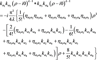
(6.5)

The exact value of the convolution we are interested in, i.e., the left hand side of (5.5), is given by the independent term in the above expansion, as it is well-known. If the reader is not familiar with this situation, see for instance [3]. We then reach

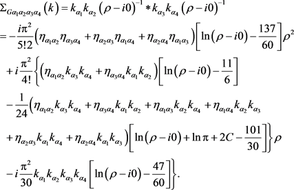(6.6)

We have to deal with 1296 diagrams of this kind.

7. Including Axions into the Picture

Axions are hypothetical elementary particles postulated by the Peccei-Quinn theory in 1977 to tackle the strong CP problem in quantum chromodynamics. If they exist and have low enough mass (within a certain range), they could be of interest as possible components of cold dark matter [15]. We include now a massive scalar field (axions) interacting with the graviton. The Lagrangian becomes

(7.1)

We can now recast the Lagrangian in the fashion

(7.2)

where

(7.3)

so that becomes the Lagrangian for the axion-graviton action

(7.4)

The new term in the interaction Hamiltonian is

(7.5)

8. The Complete Self Energy of the Graviton

The presence of axions generates a new contribution to the graviton’s self energy

(8.1)

So as to compute it we appeal to the usual integral together with the generalized Feynman-parameters. After a Wick rotation we obtain

(8.2)

where

(8.3)

After the variables-change we find

(8.4)

where

(8.5)

After evaluation of the pertinent integrals we arrive at

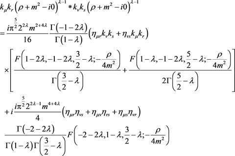
(8.6)

Self-Energy Evaluation for

We need again a Laurent’s expansion and face

(8.7)

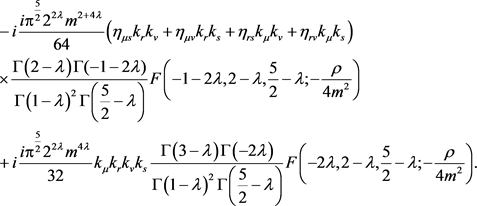
Again, the exact result for our four-dimensional convolution becomes

(8.8)

We have to deal with 9 diagrams of this kind.

Accordingly, our desired self-energy total is a combination of and.

9. Self Energy of the Axion

Here a typical term of the self-energy is:

(9.1)

In four dimensions one has

(9.2)

with the Feynman parameters used above we obtain

(9.3)

where

(9.4)

We evaluate the integral (9.3) and find

(9.5)

Self-Energy Evaluation for

Once again, we Laurent-expand, this time (9.5) around, encountering

(9.6)

The -independent term gives the exact convolution result we are looking for:

(9.7)

10. Discussion

We have developed above a quantum field theory (QFT) of Eintein’s gravity (EG), that is both unitary and finite, by appealing to the Schwinger-Feyman variational principle. We emphatically avoid the functional integral method. Our results critically depend on the use of a rather novel constraint the we introduced in defining the EG-Lagrangian. Laurent expansions were also an indispensable tool for us. As sgtated, in order to quantify the theory we appealed to the variational principle of Schwinger-Feynman’s. This process leads to just one graviton type. The underlying mathematics used in this effort has been developed by Bollini et al. [1] [2] [3] [4] [5]. This mathematics is powerful enough so as to be able to quantize non-renormalizable field theories [1] [2] [3] [4] [5]. We have evaluated here in finite and exact fashion, for the first time as far as we know, several quantities:

• the graviton’s self-energy in the EG-field. This requires full use of the theory of distributions, appealing to the possibility of creating with them a ring with divisors of zero.

• the above self-energy in the added presence of a massive scalar field (axions, for instance). Two types of diagram ensue: the original ones of the pure EG field plus the ones originated by the addition of a scalar field.

• the axion’s self-energy.

• Our central results revolve around Equation (6.6), Equation (8.8), and Equation (9.7), corresponding to the graviton’s self-energy, without and with the added presence of axions. Also, we give the axion’s self-energy.

As a final remark, we would like to point out that our formula for convolutions is a mathematical definition and not a regularization.

Conflicts of Interest

The authors declare no conflicts of interest regarding the publication of this paper.

Cite this paper

Plastino, A. and Rocca, M.C. (2020) Generalization via Ultrahyperfunctions of a Gupta-Feynman Based Quantum Field Theory of Einstein’s Gravity. Journal of Modern Physics, 11, 378-394. https://doi.org/10.4236/jmp.2020.113024

References

- 1. Bollini, C.G., Escobar, T. and Rocca, M.C. (1999) International Journal of Theoretical Physics, 38, 2315. https://doi.org/10.1023/A:1026623718239
- 2. Bollini, C.G. and Rocca, M.C. (2004) International Journal of Theoretical Physics, 43, 1019. https://doi.org/10.1023/B:IJTP.0000048599.21501.93
- 3. Bollini, C.G. and Rocca, M.C. (2004) International Journal of Theoretical Physics, 43, 59. https://doi.org/10.1023/B:IJTP.0000028850.35090.24
- 4. Bollini, C.G., Marchiano, P. and Rocca, M.C. (2007) International Journal of Theoretical Physics, 46, 3030. https://doi.org/10.1007/s10773-007-9418-y
- 5. Plastino, A. and Rocca, M.C. (2018) Journal of Physics Communications, 2, Article ID: 115029. https://doi.org/10.1088/2399-6528/aaf186
- 6. Plastino, A. and Rocca, M.C. (2019) Gupta-Feynman Based Quantum Field Theory of Einstein’s Gravity. https://www.researchgate.net/publication/336406184_Gupta-Feynman_based_Quantum_Field_Theory_of_Einstein’s_Gravity
- 7. Gupta, S.N. (1968) Proc. Pys. Soc. A, 65, 161.
- 8. Grothendieck, A. (1955) Memoirs of the American Mathematical Society, 16. https://doi.org/10.1090/memo/0016
- 9. Sebastiao e Silva, J. (1958) Mathematische Annalen, 136, 38. https://doi.org/10.1007/BF01350287
- 10. Feynman, R.P. (1963) Acta Physica Polonica, 24, 697.
- 11. Visconti, A. (1969) Quantum Field Theory. Pergamon Press, Oxford.
- 12. Delbourgo, R. and Prasad, V.B.J. (1975) Journal of Physics G: Nuclear Physics, 1, 377. https://doi.org/10.1088/0305-4616/1/4/001
- 13. Barci, D.G., Bollini, C.G. and Rocca, M.C. (1995) Il Nuovo Cimento, 108, 797. https://doi.org/10.1007/BF02731021
- 14. Kleinert, H. (2016) Particles and Quantum Fields. Free Web Version. https://pt.b-ok2.org/book/2747268/e795bchttps://doi.org/10.1142/9915
- 15. Peccei, R.D. (2008) The Strong CP Problem and Axions. In: Kuster, M., Raffelt, G. and Beltrn, B., Eds., Axions: Theory, Cosmology, and Experimental Searches, Lecture Notes in Physics, Vol. 741, Springer, Heidelberg, 3-17. https://doi.org/10.1007/978-3-540-73518-2_1