ABSTRACT

The extrapolation technique has been proved to be very powerful in improving the performance of the approximate methods by large time whether engineering or scientific problems that are handled on computers. In this paper, we investigate the efficiency of extrapolation of explicit general linear methods with Inherent Runge-Kutta stability in solving the non-stiff problems. The numerical experiments are shown for Van der Pol and Brusselator test problems to determine the efficiency of the explicit general linear methods with extrapolation technique. The numerical results showed that method with extrapolation is efficient than method without extrapolation.

Keywords:

Extrapolation Technique, General Linear Methods, Inherent Runge-Kutta Stability, Explicit Methods

1. Introduction

The two traditional numerical methods such as linear multi-step and RK methods had been studied separately to solve the problems in ordinary differential equations. General linear methods (GLMs) have been considered by Butcher as a unifying framework for both multi-value and multi-stage methods [1]. The researchers approved that these methods have a nice balanced between stability and accuracy with lower computational cost.

General linear methods are constructed by four coefficient matrices A, U, B and V utilized in partitioned $\left(s+r\right)\times \left(s+r\right)$ matrix, given by

$\left[\begin{array}{c}\begin{array}{cc}{A}_{s\times s}& U_{s\times r}\\ B_{r\times s}& V_{r\times r}\end{array}\end{array}\right]$

The coefficients of these matrices denote the connection between various numerical quantities that arise in the computation. The coefficient matrix A denotes the implementation costs of GLM methods.

Consider the initial-value problem given by

$\begin{array}{l}{y}^{\prime }\left(x\right)=f\left(y\left(x\right)\right)\mathrm{,}x\in \left[x_0\mathrm{,}X\right]\\ y\left(x_0\right)=y_0\end{array}$ (1)

The general linear methods for N-dimensional differential Equations (1) are given as follows:

$\begin{array}{l}{Y}_i={\displaystyle \underset{j=1}{\overset{s}{\sum }}}{a}_{ij}hf\left(Y_j\right)+{\displaystyle \underset{j=1}{\overset{r}{\sum }}}{u}_{ij}{y}_j^{\left[n-1\right]},i=1,2,\cdots ,s,\\ y_i^{[n]}={\displaystyle \underset{j=1}{\overset{s}{\sum }}}{b}_{ij}hf\left(Y_j\right)+{\displaystyle \underset{j=1}{\overset{r}{\sum }}}{v}_{ij}{y}_j^{\left[n-1\right]},i=1,2,\cdots ,r,\end{array}$ (2)

where $Y_i$ known as internal stage value, $f\left(Y_j\right)$ known as the identical stage derivatives, $y_i^{\left[n\right]}$ and $y_i^{\left[n-1\right]}$ are known as the incoming approximation and outgoing approximation respectively.

For more convenience, the above formula can be written in compact form as follows:

$Y^{\left[n\right]}=h\left(A\otimes I_m\right)F\left(Y^{\left[n\right]}\right)+\left(U\otimes I_m\right)y^{\left[n-1\right]},$

$y^{\left[n\right]}=h\left(B\otimes I_m\right)F\left(Y^{\left[n\right]}\right)+\left(V\otimes I_m\right)y^{\left[n-1\right]},$

where

$Y^{\left[n\right]}=\left[\begin{array}{c}{Y}_1^{\left[n\right]}\\ Y_2^{\left[n\right]}\\ ⋮\\ Y_s^{\left[n\right]}\end{array}\right],F\left(Y^{\left[n\right]}\right)=\left[\begin{array}{c}F\left(Y_1^{\left[n\right]}\right)\\ F\left(Y_2^{\left[n\right]}\right)\\ ⋮\\ F\left(Y_s^{\left[n\right]}\right)\end{array}\right],y^{\left[n-1\right]}=\left[\begin{array}{c}{y}_1^{\left[n-1\right]}\\ y_2^{\left[n-1\right]}\\ ⋮\\ y_s^{\left[n-1\right]}\end{array}\right].$

The components of input vector $y_i^{\left[n-1\right]}$ of next step satisfied as follows

$y_i^{\left[n-1\right]}={\displaystyle \underset{k=0}{\overset{p}{\sum }}}{q}_{i,k}{h}^k{y}^{\left(k\right)}\left(t_{n-1}\right)+O\left(h^{p+1}\right),i=1,\cdots ,r,$

given for some parameters $q_{i\mathrm{,}k}$ where $i=1,2,\cdots ,r$ and $k=0,1,\cdots ,p$.

The GLMs have order conditions p if the components of output vector $y_i^{\left[n\right]}$ satisfied as follows

$y_i^{\left[n\right]}={\displaystyle \underset{k=0}{\overset{p}{\sum }}}{q}_{i,k}{h}^k{y}^{\left(k\right)}\left(t_n\right)+O\left(h^{p+1}\right),i=1,\cdots ,r,$

given also for same the parameters $q_{i\mathrm{,}k}$.

The quantities $y^{\left(n\right)}\mathrm{,}{y}^{\left(n-1\right)}\mathrm{,}Y$ and $f\left(Y\right)$ of GLMs can be related as

$\left[\begin{array}{c}Y\\ y^{\left(n\right)}\end{array}\right]=\left[\begin{array}{cc}A\otimes I& U\otimes I\\ B\otimes I& V\otimes I\end{array}\right]\left[\begin{array}{c}hf\left(Y\right)\\ y^{\left(n-1\right)}\end{array}\right]$

There are some known methods that can be formulated as general linear methods given in the following [2].

First consider the RK methods given by

$\begin{array}{ccccc}0& & & & \\ \frac{1}{2}& \frac{1}{2}& & & \\ \frac{1}{2}& 0& \frac{1}{2}& & \\ 1& 0& 0& 1& \\ & \frac{1}{6}& \frac{1}{3}& \frac{1}{3}& \frac{1}{6}\end{array}$

are written as formula of GLMs as follows:

$\left[\begin{array}{c}\begin{array}{ccccc}0& 0& 0& 0& 1\\ \frac{1}{2}& 0& 0& 0& 1\\ 0& \frac{1}{2}& 0& 0& 1\\ 0& 0& 1& 0& 1\\ \frac{1}{6}& \frac{1}{3}& \frac{1}{3}& \frac{1}{6}& 1\end{array}\end{array}\right]$

Another example of Adams-Bashforth method that is given by

$y_n=y_{n-1}+h\left(\frac{3}{2}f\left(y_{n-1}\right)-\frac{1}{2}f\left(y_{n-2}\right)\right)\mathrm{,}$

can be written as formula of GLMs as follows:

$\left[\begin{array}{c}\begin{array}{cccc}0& 1& \frac{3}{2}& -\frac{1}{2}\\ 0& 1& \frac{3}{2}& -\frac{1}{2}\\ 1& 0& 0& 0\\ 0& 0& 1& 0\end{array}\end{array}\right]$

The researchers have been trying many ways to construct the efficient GLMs in solving the ordinary differential equations (ODE), such as [3]. They extended the exponential GLMs for initial value problems in solving the ordinary differential equations. They used feature of exponential, which allows deriving the order conditions of GLMs that in turn assisted in the construction of family of methods of higher order. The stability property is consistent with these methods but used the advantage of having smaller computational effort. Another example of using the effective of GLMs for solving the methods is explained by [4]. He used the GLMs for solving Volterra integro-differential equations. The article showed that GLMs are efficient in solving the nonlinear Volterra integro-differential equations. In [5], on the other hand had developed and generalized the Adams scheme which is known as Fuzzy GLMs for solving fuzzy differential problems under the generalized differentiable. They showed that the order of accuracy is more efficient than the novel scheme.

In this paper, the advantages of using the extrapolation technique with explicit GLMs methods are given for some non-stiff problems. The extrapolation technique provides one of the essential sorts of the numerical integrator to solve the ordinary differential equations within an efficient step-size control mechanism and uncomplicated variable order strategy.

The organization of this paper is as follows. Section 2 discusses the order conditions of GLMs with IRKs property, where the order conditions p considered is equal to stage order q. The construction of GLMs with IRKs property is given in Section 3. Section 4 explains the types of extrapolation technique such as active and passive. Although there are two modes in applying extrapolation, this article only considers passive extrapolation to solve some non-stiff problems such as Van der Pol and Brusselator test problems. The numerical results are given in Section 5.

2. Order Conditions

There are challenges between the researchers to construct and implement the GLMs in an easy way. Most of them consider two main assumptions in constructing these methods.

First assumption is by denoting the order condition p equal to the stage order q. The stage values satisfied as follows:

$Y^{\left[n\right]}\approx \left[\begin{array}{c}y\left(x_{n-1}+c_{1}h\right)\\ y\left(x_{n-1}+c_{2}h\right)\\ ⋮\\ y\left(x_{n-1}+c_{s}h\right)\end{array}\right]+O\left(h^{p+1}\right).$ (3)

Second assumption denotes the quantities should have a simple structure passed from step to step in order to avoid the complicated of changing step-size. Therefore, the Nordsiek form is required to present the input and output quantities.

$y^{\left[n\right]}\approx \left[\begin{array}{c}y\left(x_n\right)\\ h{y}^{\prime }\left(x_n\right)\\ ⋮\\ h^p{y}^{\left(p\right)}\left(x_n\right)\end{array}\right]+O\left(h^{p+1}\right)$ (4)

In order to describe the order condition, then the following theorem is needed [6].

Theorem 1 GLMs with coefficient matrices A, U, B and V represented in Nordsieck representation, has $p=q$ if and only if

$\exp \left(cz\right)=zA\exp \left(cz\right)+UZ+O\left(z^{p+1}\right),$

$\exp \left(z\right)Z=zB\exp \left(cz\right)+VZ+O\left(z^{p+1}\right),$

where $\exp \left(cz\right)$ indicates the vector for ith components which is equal to $\exp \left(c_{i}z\right)$. This means

$\exp \left(cz\right)=\left[\begin{array}{c}\exp \left(c_{1}z\right)\\ \exp \left(c_{2}z\right)\\ ⋮\\ \exp \left(c_{s}z\right)\end{array}\right].$

3. Construction GLMs with Inherent RK Stability

Construction GLMs with Inherent RK stability that was given by Will Wright [2] is by considering the stability of GLMs as same as RK methods, because RK methods have a good stability than other methods, such as linear multistep methods. Wright constructed Inherent RK stability (IRKs) which is a subclass of GLMs.

In order to make the stability of GLMs similar with RK methods, first consider all the eigenvalue of the stability matrix $M\left(z\right)$ equal to one, which is given by

$M\left(z\right)=V+zB{\left(I-zA\right)}^{-1}U\mathrm{,}$

and consider the stability function

The stability function can be solved by assuming, then the stability property of GLMs is similar with RK methods. Furthermore, the stability region is defined as follows:

The following definition is important to show the idea of IRKs for GLMs.

Definition 1 [2]

The general linear methods have stability as same as RK methods if its stability function satisfy the following

where denotes the rational function, which has the same significance of RK methods.

Moreover, there is another important definition necessary for the IRKS property.

Definition 2

The general linear methods, which satisfy have IRKs property if

(5)

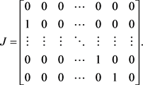
where J denotes the shifting matrix, which is given by

The following theorem discusses the GLMs with IRKs in a more practical way [7].

Theorem 2

If the general linear methods have IRKs property with stability matrix considered as

Then the stability polynomial, is defined by

Proof.

Consider another stability matrix that have the same property of the old one that is given by

(6)

By applying to the system of Equations (5) into the right side of (6)

Then, the matrix V is similar to except for the first row.

Now, by assume the matrix V has only one non-zero eigenvalue to guarantee the methods is stable, then the stability matrix has also one non-zero eigenvalue.

In [8], they gave an improved explicit type of GLMs using inherent RK methods. They gave an algorithm for the construction, described as follows:

• Choose the constant in the stability function

so that the initial value problem with stability function has stability properties and desirable accuracy;

• Choose the vector c as;

• Choose the parameters are accours in the doubly companion matrix. They are assumed that, where E is the error constant of the existing method;

• Define the following coefficients

• Find LU decomposition of the coefficient

• Consider the matrix via

Therefore, they are considered the basic coefficients of explicit GLMs with inherent RK methods as follows:

4. Extrapolation Technique

Richardson [9] [10] introduced extrapolation as a powerful technique to improve the accuracy of time integration methods of numerical analysis and to accelerate the convergence of a sequence of approximation. Extrapolation technique applied to compute quantities which relied on a parameter like a step-size or mesh. This means, the extrapolation has been successfully applied to numerical ordinary differential equations and numerical quadrature equations. Chan [11] extended the theoretical analysis of extrapolation to arbitrary RK methods for stiff ordinary differential equations. He investigated the class of symmetric RK methods which contains h²-asymptotic error expansions and generalized the concept of symmetry to composite RK methods that preserve the h²-error expansion and also create the necessary damping. These methods have same upside to increase the order by two at a time on successive extrapolations. Later, Gorgey in [12] showed that passive extrapolation of the two stage Gauss method is more efficient than the active extrapolation for solution the linear problems.

In [13], a new procedure to build stabilized explicit RK methods based on Richardson extrapolation with high order is studied. The strategy was easy and allowed deriving stabilized explicit RK methods with order as high as desired. However, for low order, the stability properties were a little shorter than other methods without this technique. They showed that methods do not suffer from propagation of errors nor internal instabilities.

Therefore, the extrapolation technique has an efficient way to improve the accuracy of GLMs with inherent RK stability. We use MATLAB code irks14-extrap.m that has extrapolation implementation of explicit GLMs with inherent RK stability.

5. Numerical Results

In this section, the results of numerical experiments obtained by the MATLAB code irks14-extrap.m are discussed. This code based on GLMs with inherent RK stability of order with extrapolation. To compare, it is also present the results obtained by the MATLAB code irks14.m. This code is based on GLMs with inherent RK stability of order, which is described in [8].

These results will show which one the most efficient methods to solve the non-stiff problems such as brusselator and Van der Pol test problems.

The first test problem is Brusselator (BRUS) which is an autocatalytic oscillating chemical reaction equation. It is a system of two ordinary differential equations which is assumed as follows

where and; it is integrated into by using .

The second test problem is Van der Pol (VDP) which is defined as follows:

where the first equation denotes the non-stiff equation while the second equation denotes stiff equation with including small. In order to solve the non-stiff problem, then considered here equal to one. The initial values of VDP given as follows:

Figure 1 shows the numerical results on BRUS test problem. From the figure, we can see the extrapolation of GLMs with inherent RK stability of order four gives better efficiency than same methods without extrapolation. Furthermore, the numerical results given in Figure 2 show the extrapolation of GLMs with inherent RK stability of order four gives also better efficiency than same methods without extrapolation for VDP test problem.

6. Conclusions

In this paper, we discuss some issues related to developing the construction of Explicit general linear methods with inherent Runge-stability for numerical solution of non-stiff differential equations. These issues include the application of extrapolation technique to this base method. As we can see from the results in this paper, the extrapolation technique with explicit GLMs with inherent RK stability of order four on BRUS and VDP test problems, both give better efficiency than explicit GLMs without extrapolation.

Future work will involve verifying the efficiency of extrapolation of explicit GLMs with inherent RK stability for higher order for numerical solution of non stiff differential equations as well as the implicit GLMs for stiff equations.

Acknowledgements

The authors would like to extend their gratitude to the Sultan Idris Education University especially the Research Management and Innovation Center for providing the research grant GPU, Vote No: 2018-0149-102-01.

Conflicts of Interest

The authors declare no conflicts of interest regarding the publication of this paper.

Cite this paper

Kadhim, A.J. and Gorgey, A. (2019) Extrapolation of GLMs with IRKS Property to Solve the Ordinary Differential Equations. American Journal of Computational Mathematics, 9, 251-260. https://doi.org/10.4236/ajcm.2019.94019

References

- 1. Butcher, J.C. (2009) General Linear Methods for Ordinary Differential Equations. Mathematics and Computers in Simulation, 79, 1834-1845. https://doi.org/10.1016/j.matcom.2007.02.006
- 2. Wright, W. (2002) General Linear Methods with Inherent Runge-Kutta Stability. Ph.D. Thesis, the University of Auckland, New Zealand.
- 3. Bazuaye, F.E. and Osisiogu, U.A. (2017) A New Approach to Constructing Extended Exponential General Linear Methods for Initial Value Problems in Ordinary Differential Equations. International Journal of Advances in Mathematics, 5, 44-54.
- 4. Mahdi, H., Abdi, A. and Hojjati, G. (2018) Efficient General Linear Methods for a Class of Volterra Integro-Differential Equations. Applied Numerical Mathematics, 127, 95-109. https://doi.org/10.1016/j.apnum.2018.01.001
- 5. Farzi, J. and Mordai, A. (2018) Fuzzy General Linear Methods. arXiv:1812.03394.
- 6. Cardone, A., Jackiewicz, Z., Verner J.H. and Welfert, B. (2015) Order Conditions for General Linear Methods. Journal of Computational and Applied Mathematics, 290, 44-64. https://doi.org/10.1016/j.cam.2015.04.042
- 7. Butcher, J.C. (2001) General Linear Methods for Stiff Differential Equations. BIT Numerical Mathematics, 41, 240-264. https://doi.org/10.1023/A:1021986222073
- 8. Abdi, A. and Jackiewicz, Z. (2019) Towards a Code for Nonstiff Differential Systems Based on General Linear Methods with Inherent Runge-Kutta Stability. Applied Numerical Mathematics, 136, 103-121. https://doi.org/10.1016/j.apnum.2018.10.001
- 9. Richardson, L.F. (1911) The Approximate Arithmetical Solution by Finite Differences of Physical Problems Involving Differential Equations, with an Application to the Stresses in a Masonry Dam. Philosophical Transactions of the Royal Society A, 210, 307-357. https://doi.org/10.1098/rsta.1911.0009
- 10. Richardson, L.F. (1927) The Deferred Approach to the Limit. Philosophical Transactions of the Royal Society A, 226, 299-349. https://doi.org/10.1098/rsta.1927.0008
- 11. Chan, R.P.K. (1996) A-Stability of Implicit Runge-Kutta Extrapolations. Applied Numerical Mathematics, 22, 179-203. https://doi.org/10.1016/S0168-9274(96)00031-1
- 12. Gorgey, A. (2012) Extrapolation of Symmetrized Runge-Kutta Methods. Ph.D. Thesis, the University of Auckland, New Zealand.
- 13. Martín-Vaquero, J. and Kleefeld, B. (2016) Extrapolated Stabilized Explicit Runge-Kutta. Methods Journal of Computational Physics, 326, 141-155. https://doi.org/10.1016/j.jcp.2016.08.042