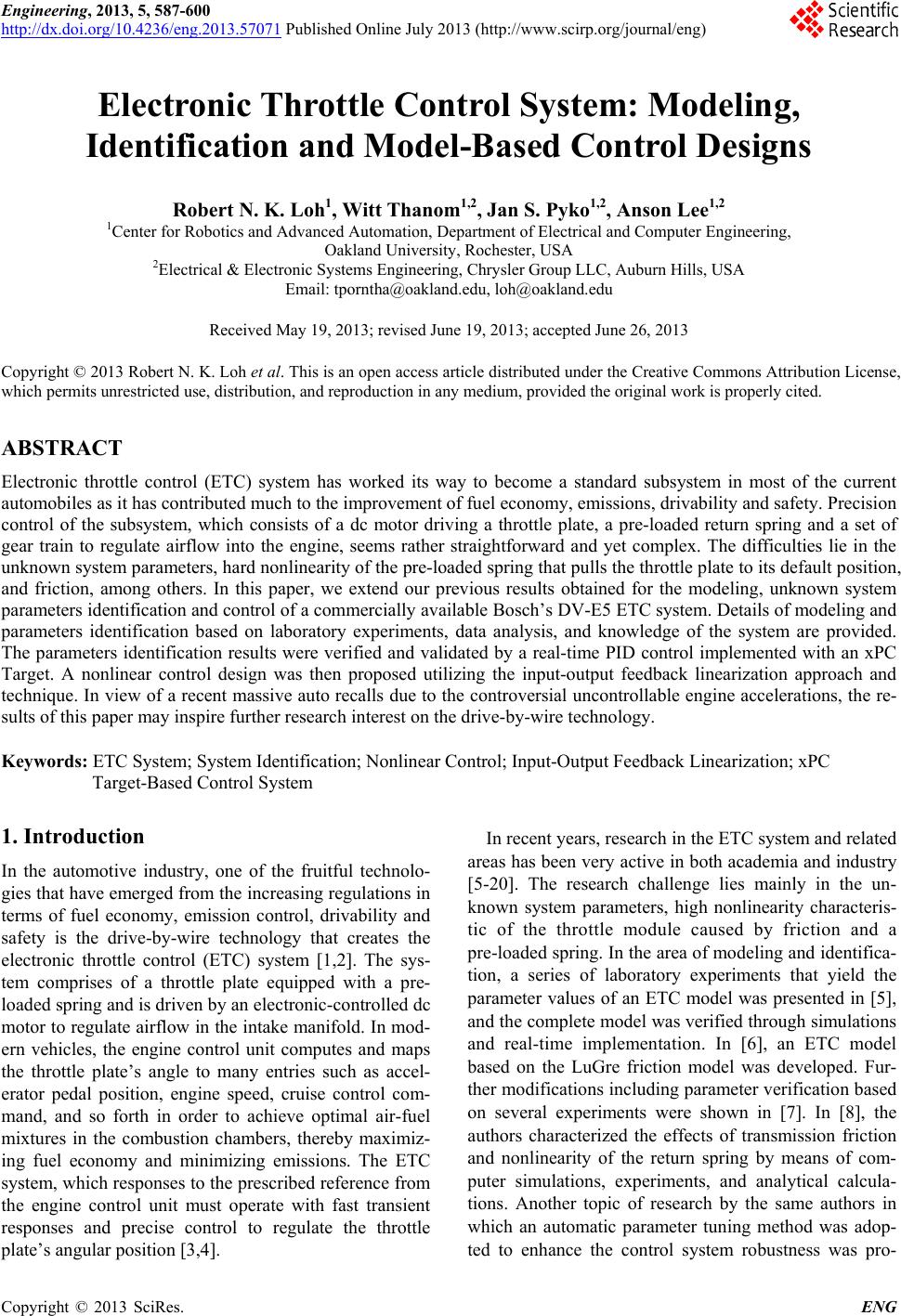
Engineering, 2013, 5, 587-600
http://dx.doi.org/10.4236/eng.2013.57071 Published Online July 2013 (http://www.scirp.org/journal/eng)
Electronic Throttle Control System: Modeling,
Identification and Model-Based Control Designs
Robert N. K. Loh1, Witt Thanom1,2, Jan S. Pyko1,2, Anson Lee1,2
1Center for Robotics and Advanced Automation, Department of Electrical and Computer Engineering,
Oakland University, Rochester, USA
2Electrical & Electronic Systems Engineering, Chrysler Group LLC, Auburn Hills, USA
Received May 19, 2013; revised June 19, 2013; accepted June 26, 2013
Copyright © 2013 Robert N. K. Loh et al. This is an open access article distributed under the Creative Commons Attribution License,
which permits unrestricted use, distribution, and reproduction in any medium, provided the original work is properly cited.
ABSTRACT
Electronic throttle control (ETC) system has worked its way to become a standard subsystem in most of the current
automobiles as it has contributed much to the improvement of fuel economy, emissions, drivability and safety. Precision
control of the subsystem, which consists of a dc motor driving a throttle plate, a pre-loaded return spring and a set of
gear train to regulate airflow into the engine, seems rather straightforward and yet complex. The difficulties lie in the
unknown system parameters, hard nonlinearity of the pre-loaded spring that pulls the throttle plate to its default position,
and friction, among others. In this paper, we extend our previous results obtained for the modeling, unknown system
parameters identification and control of a commercially available Bosch’s DV-E5 ETC system. Details of modeling and
parameters identification based on laboratory experiments, data analysis, and knowledge of the system are provided.
The parameters identification results were verified and validated by a real-time PID control implemented with an xPC
Target. A nonlinear control design was then proposed utilizing the input-output feedback linearization approach and
technique. In view of a recent massive auto recalls due to the controversial uncontrollable engine accelerations, the re-
sults of this paper may inspire further research interest on the drive-by-wire technology.
Keywords: ETC System; System Identification; Nonlinear Control; Input-Output Feedback Linearization; xPC
Target-Based Control System
1. Introduction
In the automotive industry, one of the fruitful technolo-
gies that have emerged from the increasing regulations in
terms of fuel economy, emission control, drivability and
safety is the drive-by-wire technology that creates the
electronic throttle control (ETC) system [1,2]. The sys-
tem comprises of a throttle plate equipped with a pre-
loaded spring and is driven by an electronic-controlled dc
motor to regulate airflow in the intake manifold. In mod-
ern vehicles, the engine control unit computes and maps
the throttle plate’s angle to many entries such as accel-
erator pedal position, engine speed, cruise control com-
mand, and so forth in order to achieve optimal air-fuel
mixtures in the combustion chambers, thereby maximiz-
ing fuel economy and minimizing emissions. The ETC
system, which responses to the prescribed reference from
the engine control unit must operate with fast transient
responses and precise control to regulate the throttle
plate’s angular position [3,4].
In recent years, research in the ETC system and related
areas has been very active in both academia and industry
[5-20]. The research challenge lies mainly in the un-
known system parameters, high nonlinearity characteris-
tic of the throttle module caused by friction and a
pre-loaded spring. In the area of modeling and identifica-
tion, a series of laboratory experiments that yield the
parameter values of an ETC model was presented in [5],
and the complete model was verified through simulations
and real-time implementation. In [6], an ETC model
based on the LuGre friction model was developed. Fur-
ther modifications including parameter verification based
on several experiments were shown in [7]. In [8], the
authors characterized the effects of transmission friction
and nonlinearity of the return spring by means of com-
puter simulations, experiments, and analytical calcula-
tions. Another topic of research by the same authors in
which an automatic parameter tuning method was adop-
ted to enhance the control system robustness was pro-
C
opyright © 2013 SciRes. ENG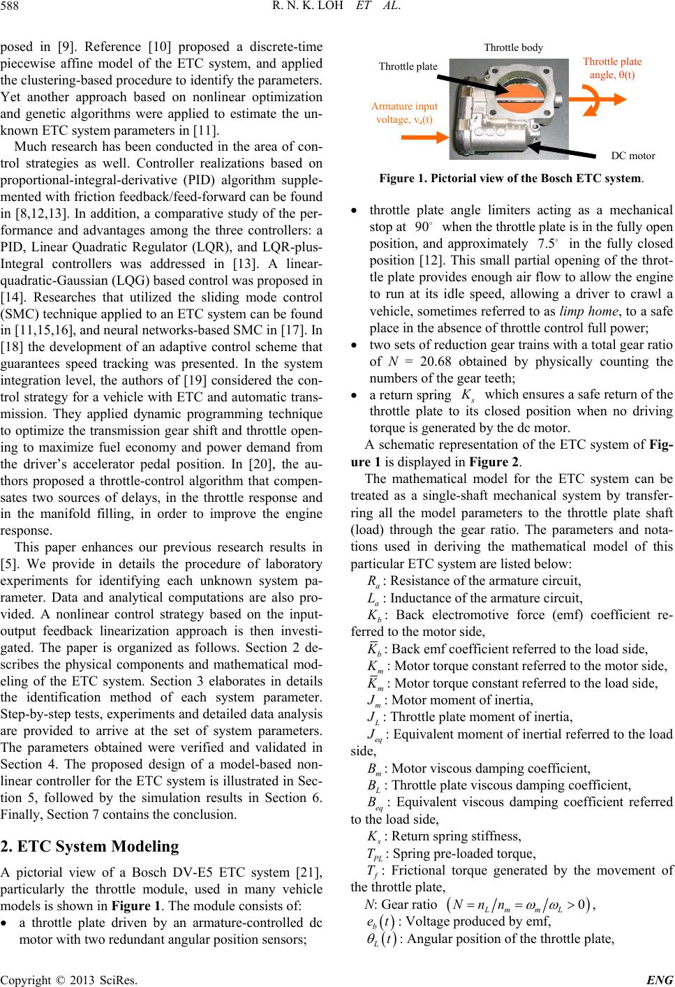

R. N. K. LOH ET AL. 588
posed in [9]. Reference [10] proposed a discrete-time
piecewise affine model of the ETC system, and applied
the clustering-based procedure to identify the parameters.
Yet another approach based on nonlinear optimization
and genetic algorithms were applied to estimate the un-
known ETC system parameters in [11].
Much research has been conducted in the area of con-
trol strategies as well. Controller realizations based on
proportional-integral-derivative (PID) algorithm supple-
mented with friction feedback/feed-forward can be found
in [8,12,13]. In addition, a comparative study of the per-
formance and advantages among the three controllers: a
PID, Linear Quadratic Regulator (LQR), and LQR-plus-
Integral controllers was addressed in [13]. A linear-
quadratic-Gaussian (LQG) based control was proposed in
[14]. Researches that utilized the sliding mode control
(SMC) technique applied to an ETC system can be found
in [11,15,16], and neural networks-based SMC in [17]. In
[18] the development of an adaptive control scheme that
guarantees speed tracking was presented. In the system
integration level, the authors of [19] considered the con-
trol strategy for a vehicle with ETC and automatic trans-
mission. They applied dynamic programming technique
to optimize the transmission gear shift and throttle open-
ing to maximize fuel economy and power demand from
the driver’s accelerator pedal position. In [20], the au-
thors proposed a throttle-control algorithm that compen-
sates two sources of delays, in the throttle response and
in the manifold filling, in order to improve the engine
response.
This paper enhances our previous research results in
[5]. We provide in details the procedure of laboratory
experiments for identifying each unknown system pa-
rameter. Data and analytical computations are also pro-
vided. A nonlinear control strategy based on the input-
output feedback linearization approach is then investi-
gated. The paper is organized as follows. Section 2 de-
scribes the physical components and mathematical mod-
eling of the ETC system. Section 3 elaborates in details
the identification method of each system parameter.
Step-by-step tests, experiments and detailed data analysis
are provided to arrive at the set of system parameters.
The parameters obtained were verified and validated in
Section 4. The proposed design of a model-based non-
linear controller for the ETC system is illustrated in Sec-
tion 5, followed by the simulation results in Section 6.
Finally, Section 7 contains the conclusion.
2. ETC System Modeling
A pictorial view of a Bosch DV-E5 ETC system [21],
particularly the throttle module, used in many vehicle
models is shown in Figure 1. The module consists of:
 a throttle plate driven by an armature-controlled dc
motor with two redundant angular position sensors;
Throttle body
DC motor
Armature input
voltage, v
a
(t)
Throttle plateThrottle plate
angle, (t)
Figure 1. Pictorial view of the Bosch ETC system.
 throttle plate angle limiters acting as a mechanical
stop at 90 when the throttle plate is in the fully open
position, and approximately 7.5 in the fully closed
position [12]. This small partial opening of the throt-
tle plate provides enough air flow to allow the engine
to run at its idle speed, allowing a driver to crawl a
vehicle, sometimes referred to as limp home, to a safe
place in the absence of throttle control full power;
 two sets of reduction gear trains with a total gear ratio
of N = 20.68 obtained by physically counting the
numbers of the gear teeth;
 a return spring
s
K
which ensures a safe return of the
throttle plate to its closed position when no driving
torque is generated by the dc motor.
A schematic representation of the ETC system of Fig-
ure 1 is displayed in Figure 2.
The mathematical model for the ETC system can be
treated as a single-shaft mechanical system by transfer-
ring all the model parameters to the throttle plate shaft
(load) through the gear ratio. The parameters and nota-
tions used in deriving the mathematical model of this
particular ETC system are listed below:
a
R
L: Resistance of the armature circuit,
a: Inductance of the armature circuit,
b
K
: Back electromotive force (emf) coefficient re-
ferred to the motor side,
b
K
: Back emf coefficient referred to the load side,
m
K
: Motor torque constant referred to the motor side,
m
K
: Motor torque constant referred to the load side,
m
J
: Motor moment of inertia,
L
J
: Throttle plate moment of inertia,
eq
J
: Equivalent moment of inertial referred to the load
side,
m
B: Motor viscous damping coefficient,
L
B: Throttle plate viscous damping coefficient,
eq : Equivalent viscous damping coefficient referred
to the load side,
B
s
K
: Return spring stiffness,
P
L
T
T: Spring pre-loaded torque,
f: Frictional torque generated by the movement of
the throttle plate,
N: Gear ratio


0
Lmm L
Nnn 

,


b
et: Voltage produced by emf,


t 
L: Angular position of the throttle plate,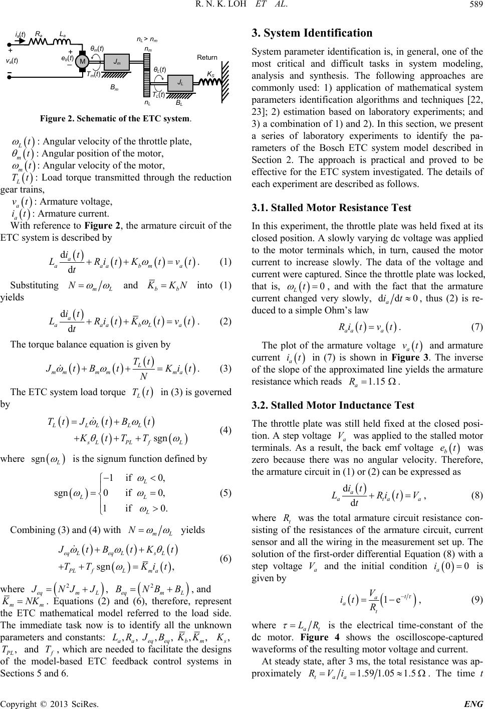

R. N. K. LOH ET AL. 589
Bm
nm θm(t)
nL
va(t)
KS
M Jm
+
nL > nm
Return
eb
(
t
)
+
_
JL
La ia(t) Ra
BL
θL(t)
T
m
(
t
)
TL(t)
Figure 2. Schematic of the ETC system.

Lt


t 
: Angular velocity of the throttle plate,
m

t 
: Angular position of the motor,
m

Tt: Angular velocity of the motor,
L: Load torque transmitted through the reduction
gear trains,

a
vt

it: Armature voltage,
a
With reference to Figure 2, the armature circuit of the
ETC system is described by
: Armature current.
  
d
d
a
aaabm
it
LRitKtv
t
  
a
t . (1)
Substituting mL N

  and bb
K
KN into (1)
yields
  
d
d
a
aaabL
it
LRitKtv
t
  
a
t. (2)
The torque balance equation is given by
  
L
mm mmma
Tt
J
tB tKit
N
 
. (3)
The ETC system load torque in (3) is governed
by

L
Tt






 
sgn
LLLLL
s
LPLf
TtJt Bt
KtTT

L





(4)
where

sgn
L

is the signum function defined by

1 if 0,
sgn0 if 0,
1 if 0.
L
L
L










L
 (5)
Combining (3) and (4) with mL
N

  yields






sgn ,
eqLeqLs L
PLfLm a
J
tBtK t
TT Kit



 

(6)
where

2
eqm L
J
NJ J, , and

2
eqm L
BNBB
mm
3. System Identification
System parameter identification is, in general, one of the
most critical and difficult tasks in system modeling,
analysis and synthesis. The following approaches are
commonly used: 1) application of mathematical system
parameters identification algorithms and techniques [22,
23]; 2) estimation based on laboratory experiments; and
3) a combination of 1) and 2). In this section, we present
a series of laboratory experiments to identify the pa-
rameters of the Bosch ETC system model described in
Section 2. The approach is practical and proved to be
effective for the ETC system investigated. The details of
each experiment are described as follows.
3.1. Stalled Motor Resistance Test
In this experiment, the throttle plate was held fixed at its
closed position. A slowly varying dc voltage was applied
to the motor terminals which, in turn, caused the motor
current to increase slowly. The data of the voltage and
current were captured. Since the throttle plate was locked,
that is,


0
Lt


, and with the fact that the armature
current changed very slowly, dd 0
a
it, thus (2) is re-
duced to a simple Ohm’s law


aaa
Ri tvt

. (7)
The plot of the armature voltage and armature
current

a
vt


a
it in (7) is shown in Figure 3. The inverse
of the slope of the approximated line yields the armature
resistance which reads 1.15
a
R

.
3.2. Stalled Motor Inductance Test
The throttle plate was still held fixed at the closed posi-
tion. A step voltage a was applied to the stalled motor
terminals. As a result, the back emf voltage
V


b
et was
zero because there was no angular velocity. Therefore,
the armature circuit in (1) or (2) can be expressed as


d
d
a
ata
it
LRit
t
a
V , (8)
where t was the total armature circuit resistance con-
sisting of the resistances of the armature circuit, current
sensor and all the wiring in the measurement set up. The
solution of the first-order differential Equation (8) with a
step voltage and the initial condition
R
a
V


00
a
i

is
given by


1e
t
a
at
V
it R



 , (9)
K
NK. Equations (2) and (6), therefore, represent
the ETC mathematical model referred to the load side.
The immediate task now is to identify all the unknown
parameters and constants: ,,
aa
LR ,,
eq eq
J
B,,
bm
K
K ,
s
K
,
P
L
T and
f
T, which are needed to facilitate the designs
of the model-based ETC feedback control systems in
Sections 5 and 6.
where at LR


is the electrical time-constant of the
dc motor. Figure 4 shows the oscilloscope-captured
waveforms of the resulting motor voltage and current.
At steady state, after 3 ms, the total resistance was ap-
proximately 1.591.051.5
taa
RVi

. The time t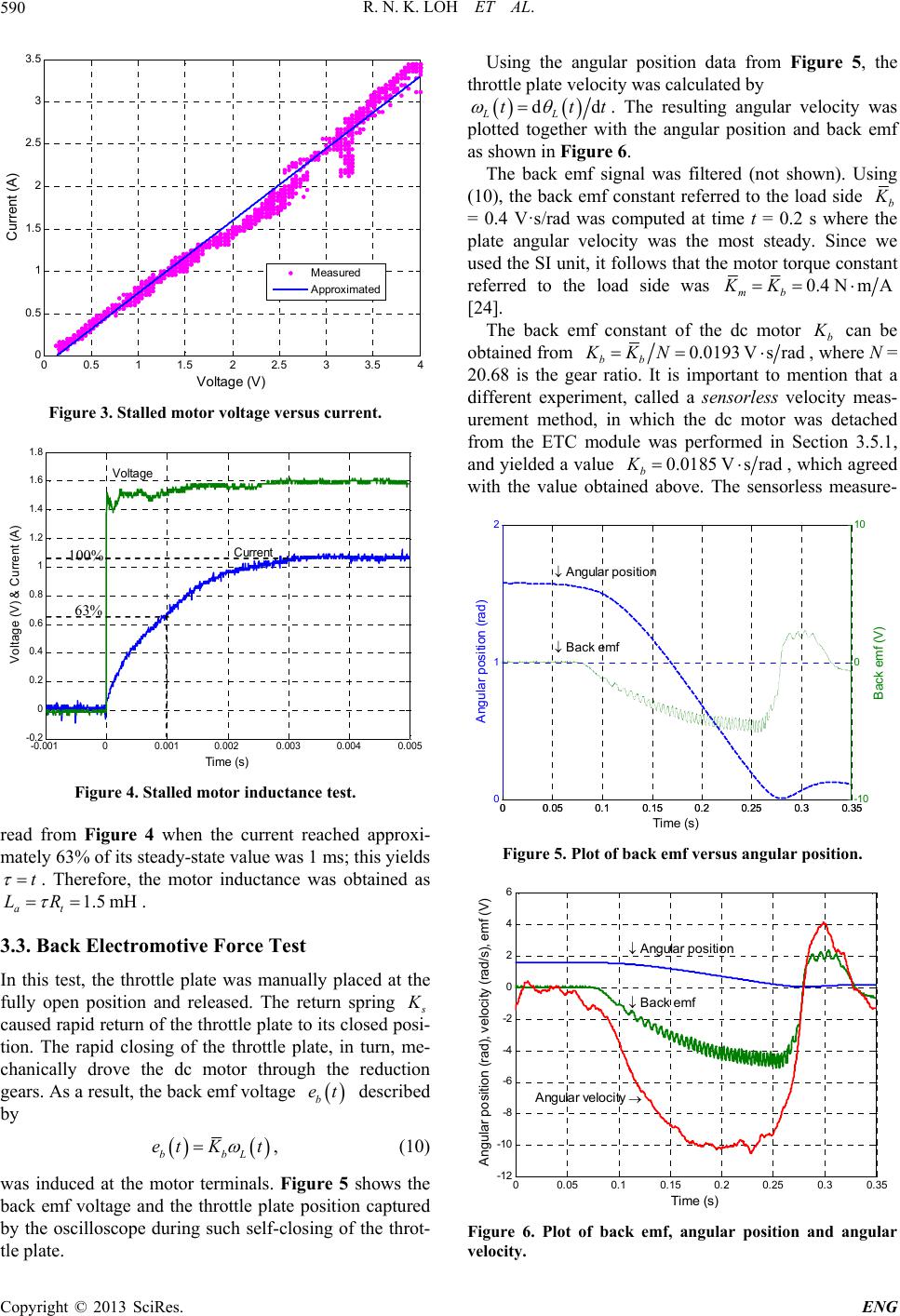

R. N. K. LOH ET AL. 590
00.5 11.5 22.5 33.5 4
0
0.5
1
1.5
2
2.5
3
3.5
Volta ge ( V)
Current (A)
Measured
Approximated
Figure 3. Stalled motor voltage versus current.
-0.001 0 0.001 0.002 0.003 0.0040.005
-0.2
0
0. 2
0. 4
0. 6
0. 8
1
1. 2
1. 4
1. 6
1. 8
Time (s)
Voltage (V) & Current (A)
Voltage
Current
100%
63%
Figure 4. Stalled motor inductance te st.
read from Figure 4 when the current reached approxi-
mately 63% of its steady-state value was 1 ms; this yields
t

. Therefore, the motor inductance was obtained as
1.5 mH
at
LR

 .
3.3. Back Electromotive Force Test
In this test, the throttle plate was manually placed at the
fully open position and released. The return spring
s
K
caused rapid return of the throttle plate to its closed posi-
tion. The rapid closing of the throttle plate, in turn, me-
chanically drove the dc motor through the reduction
gears. As a result, the back emf voltage described
by

b
et
 
bbL
tKe  t, (10)
was induced at the motor terminals. Figure 5 shows the
back emf voltage and the throttle plate position captured
by the oscilloscope during such self-closing of the throt-
tle plate.
Using the angular position data from Figure 5, the
throttle plate velocity was calculated by




d
LL
tt  dt. The resulting angular velocity was
plotted together with the angular position and back emf
as shown in Figure 6.
The back emf signal was filtered (not shown). Using
(10), the back emf constant referred to the load side b
K
= 0.4 V·s/rad was computed at time t = 0.2 s where the
plate angular velocity was the most steady. Since we
used the SI unit, it follows that the motor torque constant
referred to the load side was 0.4 NmA
mb
KK
[24].
The back emf constant of the dc motor b
K
can be
obtained from 0.0193 Vsrad
bb
KKN , where N =
20.68 is the gear ratio. It is important to mention that a
different experiment, called a sensorless velocity meas-
urement method, in which the dc motor was detached
from the ETC module was performed in Section 3.5.1,
and yielded a value 0.0185 Vsrad
b
K

, which agreed
with the value obtained above. The sensorless measure-
00.05 0.10.15 0.2 0.25 0.3 0.35
0
1
2
Time (s)
Angular position (r a d)
 Back emf
 An gular posit ion
00.05 0.10.15 0.2 0.25 0.3 0.35
-10
0
10
Back emf (V)
Figure 5. Plot of back emf versus angular position.
00.05 0.10.15 0.2 0.250.30.35
-12
-10
-8
-6
-4
-2
0
2
4
6
Time (s)
Angular position ( r ad) , v elocity ( r ad/s ) , em f ( V)
 Bac k emf
 An gular position
Angular velocity 
Figure 6. Plot of back emf, angular position and angular
velocity.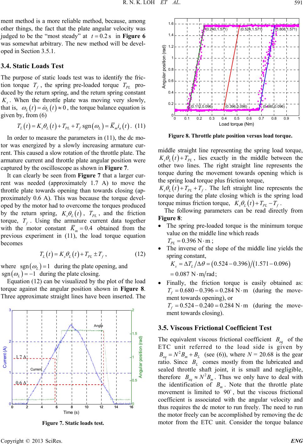

R. N. K. LOH ET AL. 591
ment method is a more reliable method, because, among
other things, the fact that the plate angular velocity was
judged to be the “most steady” at in Figure 6
was somewhat arbitrary. The new method will be devel-
oped in Section 3.5.1.
0.2 st
3.4. Static Loads Test
The purpose of static loads test was to identify the fric-
tion torque
f
T, the spring pre-loaded torque
P
L pro-
duced by the return spring, and the return spring constant
T
s
K
. When the throttle plate was moving very slowly,
that is, , the torque balance equation is
given by, from (6)

t

0
LL
t  

 


sgn
LsLPLfLma
TtKt TTKit   . (11)
In order to measure the parameters in (11), the dc mo-
tor was energized by a slowly increasing armature cur-
rent. This caused a slow rotation of the throttle plate. The
armature current and throttle plate angular position were
captured by the oscilloscope as shown in Figure 7.
It can clearly be seen from Figure 7 that a larger cur-
rent was needed (approximately 1.7 A) to move the
throttle plate towards opening than towards closing (ap-
proximately 0.6 A). This was because the torque devel-
oped by the motor had to overcome the torques produced
by the return spring,

sL
K
t  ,
P
L, and the friction
torque,
T
f
T. Using the armature current data together
with the motor constant 0.4
m obtained from the
previous experiment in (11), the load torque equation
becomes
K
 
L
sLPL f
TtKt TT  , (12)
where during the plate opening, and
during the plate closing.

sgn 1
L
 

1
Lsgn

Equation (12) can be visualized by the plot of the load
torque against the angular position shown in Figure 8.
Three approximate straight lines have been inserted. The
0 2 4 6810 12 1416
0
1
2
3
Time (s)
Current (A )
Current
Angle
0 2 4 6810 12 1416
0
0. 5
1
1. 5
2
Angular position (rad)
1.7 A
0.6 A
00.1 0.20.3 0.40.5 0.6 0.7 0.8 0.91
0
0.2
0.4
0.6
0.8
1
1.2
1.4
1.6
Load tor q ue (Nm)
Angular position ( r ad)
(0.112,0.096) (0.396,0.096)(0.680,0.096)
(0.240,1.571)(0.524,1.571) (0.808,1.571)
Figure 8. Throttle plate position versus load torque.
iddle straight line representing the spring load torque, m


s
LPL
K
tT  , lies exactly in the middle between the
es. The right straight line represents the
torque during the movement towards opening which is
the spring load torque plus friction torque,
other two lin


s
LPLf
K
tT T 

. The left straight line re
plate closing which is the spring load
torque minus friction torque,
presents the
torque during the


s
LPLf
K
tT T  .
The following parameters tly can be read direcfrom
Fi
ng pre-loaded torque is the minimum torque
gure 8:
 The spri
value on the middle line which reads
0.396 Nm
PL
T

;
 of the middle line yields the The inverse of the slope
spring constant,

 
0.5240.3961.571 0.096
0.087Nmrad;
sL
KT   

 Finally, the friction torque is easily obtained as:
0.6800.3960.284Nm
f
T

  (during the move-
0.5240.2400.284NT
ment towards opening), or
m
f

 
ment towards closing).
(during the move-
3.5. Viscous Frictional Coefficient Test
of the The equivalent viscous frictional coefficient eq B
ETC unit referred to the load side is given by
2
eqmL
BNBB

 (see (6)), where N = 20.68 is the gear
ratio. Since
L
B
fication
comes mostly from the lubricated and
sealed throttle shaft joint, it is small and negligible,
therefore 2
eq m
BNB. Thus we only have to deal with
the identim B. Note that the throttle plate
movement is limited t90, but the viscous frictional
coefficient is associated h the angular velocity and
thus requires the dc motor to run freely. The need to run
the motor freely can be accomplished by removing the dc
motor from the ETC unit. Consider the torque balance
of
o
wit
Figure 7. Static loads test.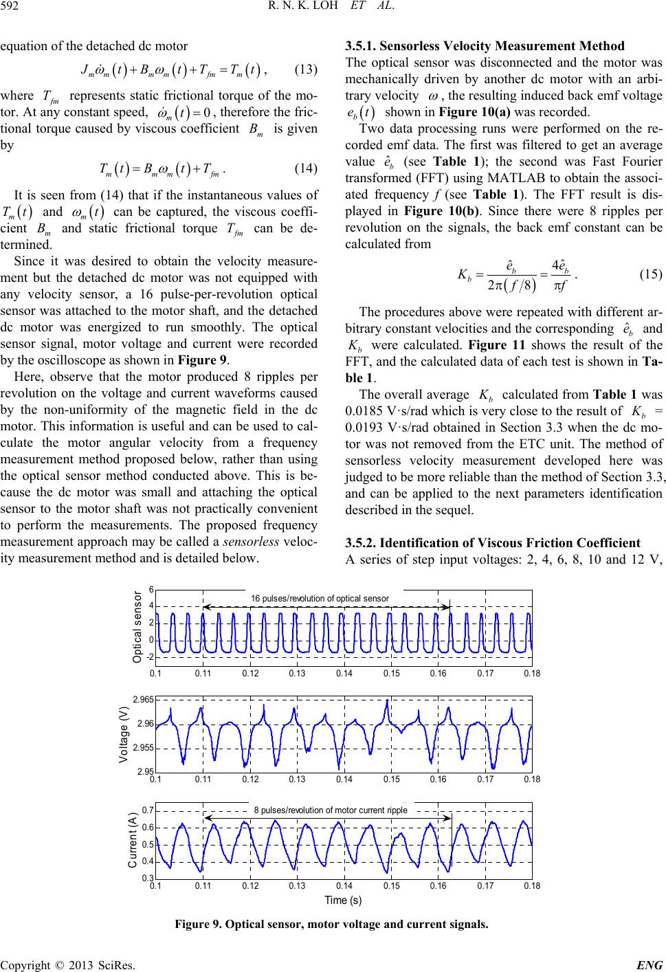

R. N. K. LOH ET AL. 592
3.5.1. Sensorless Velocity Measurement Method equation of the detached dc motor
The optical sensor was disconnected and the motor was
mechanically driven by another dc motor with an arbi-
trary velocity

, the resulting induced back emf voltage


b
et shown in Figure 10(a) was recorded.






mmmmfm m
J
tB t  
T Tt
, (13)
where
f
m
T
y
represents static frictional torque of the mo-
tor. At anconstant speed,


0
mt
 
, therefore the fric-
tional torque caused by visccient m B is given
by
ous coeffiTwo data processing runs were performed on the re-
corded emf data. The first was filtered to get an average
value (see Table 1); the second was Fast Fourier
transformed (FFT) using MATLAB to obtain the associ-
ated frequency f (see Table 1). The FFT result is dis-
played in Figure 10(b). Since there were 8 ripples per
revolution on the signals, the back emf constant can be
calculated from
ˆb
e



mmm
TtBtT  .
fm
(14)
It is seen from (14) that if the instantaneous values of

t and

mt
 can be captured, the viscous coeffi-
m
B anic frictional torque
m
T
cient d stat
f
m
T can be de-
termin
Since it
ed.
was desired to obtain the velocity measure-
m
ripples per
re

ˆˆ 4
28
b
be
Kff 


b
e
. (15)
ent but the detached dc motor was not equipped with
any velocity sensor, a 16 pulse-per-revolution optical
sensor was attached to the motor shaft, and the detached
dc motor was energized to run smoothly. The optical
sensor signal, motor voltage and current were recorded
by the oscilloscope as shown in Figure 9.
Here, observe that the motor produced 8
The procedures above were repeated with different ar-
bitrary constant velocities and the corresponding and
b
ˆb e
K
were calculated. Figure 11 shows the result of the
FFT, and the calculated data of each test is shown in Ta-
ble 1.
volution on the voltage and current waveforms caused
by the non-uniformity of the magnetic field in the dc
motor. This information is useful and can be used to cal-
culate the motor angular velocity from a frequency
measurement method proposed below, rather than using
the optical sensor method conducted above. This is be-
cause the dc motor was small and attaching the optical
sensor to the motor shaft was not practically convenient
to perform the measurements. The proposed frequency
measurement approach may be called a sensorless veloc-
ity measurement method and is detailed below.
The overall average b
K
calculated from Table 1 was
0.0185 V·s/rad which is very close to the result of b
K
=
0.0193 V·s/rad obtained in Section 3.3 when the dc mo-
tor was not removed from the ETC unit. The method of
sensorless velocity measurement developed here was
judged to be more reliable than the method of Section 3.3,
and can be applied to the next parameters identification
described in the sequel.
3.5.2. Identification of Viscous Friction Coefficient
A series of step input voltages: 2, 4, 6, 8, 10 and 12 V,
0.10.11 0.120.13 0.14 0.150.16 0.170.18
-2
0
2
4
6
Optical sensor
0.10.11 0.120.13 0.14 0.150.16 0.170.18
2.95
2.955
2.96
2.965
Voltage (V)
0.10.11 0.120.13 0.14 0.150.16 0.170.18
0.3
0.4
0.5
0.6
0.7
Time (s)
Current (A)
16 puls es/ revol ut i on of opti c al s ensor
8 pulses/revoluti on of motor c urrent ri pple
Figure 9. Optical sensor, motor voltage and current signals.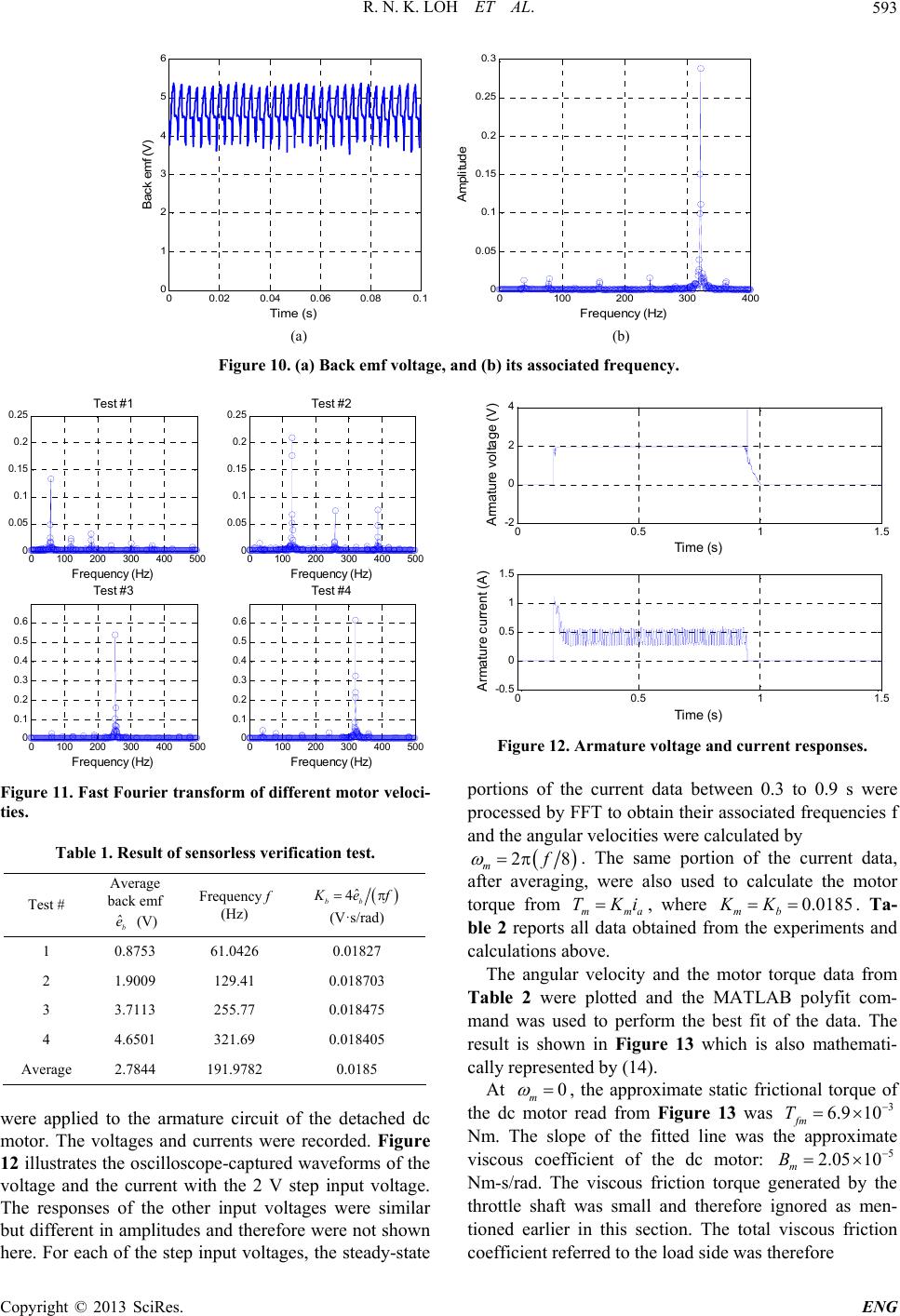

R. N. K. LOH ET AL. 593
00.02 0.04 0.06 0.080.1
0
1
2
3
4
5
6
Time (s)
Back emf (V)
0100 200300400
0
0.05
0.1
0.15
0.2
0.25
0.3
Frequ ency ( H z)
Amplitude
(a) (b)
Figure 10. (a) Back emf voltage, and (b) its associated frequency.
0100 200 300 400 500
0
0.05
0.1
0.15
0.2
0.25
Frequency (Hz)
Test #1
0100 200 300 400 500
0
0.05
0.1
0.15
0.2
0.25
Frequency (Hz)
Test #2
0100 200 300 400 500
0
0.1
0.2
0.3
0.4
0.5
0.6
Frequency (Hz)
Test #3
0100 200 300 400 500
0
0.1
0.2
0.3
0.4
0.5
0.6
Frequency (Hz)
Test #4
Figure 11. Fast Fourier transform of different motor veloc
Table 1. Result of sensorless verification test.
Test # Frequency f
i-
ties.
Average
back emf
ˆb
e (V) (Hz)


ˆ
4
bb
K
ef

(V·s/rad)
1 0.8753 61.0426 0.01827
2 1.9009 129.41 0.018703
3 3.7113 255.77 0.018475
4 4.6501 321.69 0.018405
Avge 1 era2.7844 91.97820.0185
ere applied to the armature circuit of the detached dc w
motor. The voltages and currents were recorded. Figure
12 illustrates the oscilloscope-captured waveforms of the
voltage and the current with the 2 V step input voltage.
The responses of the other input voltages were similar
but different in amplitudes and therefore were not shown
here. For each of the step input voltages, the steady-state
00.5 11.5
-2
0
2
4
Time (s)
Arm atur e volt ag)e (V
1. 5
00.5 11.5
-0.5
0
0. 5
1
Time (s)
Armature current (A)
Figure 12. Armature voltage and current responses.
portere
rocessed by FFT to obtain their associated frequencies f
ions of the current data between 0.3 to 0.9 s w
p
and the angular velocities were calculated by


28
mf
  . The same portion of the current data,
after averaging, were also used to calculate
mma
Ki
the motor
torque from T

, where 0.0185
mb
KK. Ta-
ble 2 reports all data obtained from the experiments and
calculations ab
The angular velocity and the motor torque data from
Table 2 were plott
ove.
ed and the MATLAB polyfit com-
mand was used to perform the best fit of the data. The
result is shown in Figure 13 which is also mathemati-
cally represented by (14).
At 0
m


, the approximate static frictional torque of
the dc motor read from Figure 13 was 3
6.9 10Tfm


5
2.05 10
Nm. Tpe of the fitted line was the approximate
viscous coefficient of the dc motor: m B
he slo


Nm-s/rad. The viscous friction torque generated by the
throttle shaft was small and therefore ig-
tioned earlier in this section. The total viscous friction
coefficient referred to the load side was therefore
nored as men

R. N. K. LOH ET AL. 594
Table 2. Result of viscous friction coefficient test.
Step Angular input
ltage
FFT
Frequency velocity vo f (V) (Hz) m

(rad/s)
Average Mo
measured
to
torque
cu
r
rrent a i (A)
m
T
(N·m)
2 95.2 74.80 0.405 0.0075
4 211.2 165.90 0.576
6 334.6 262.76 0.688 0.0127
8 457.9 359.61 0.813 0.0150
10 580.0 455.51 0.903 0.0167
12 704.5 553.33 0.934 0.0172
0.0106
00.02 0.040.06 0.080.10.12 0.140.16 0.18 0.2
-6
-4
-2
0
emf (V )
00.02 0.040.06 0.080.10.12 0.140.16 0.18 0.2
-10
-5
0
Velocity (rad/s)
00.02 0.040.06 0.080.10.12 0.140.16 0.18 0.2
-100
0
100
Acceleration (rad/s
2
)
00.02 0.040.06 0.080.10.12 0.140.16 0.18 0.2
-0.4
-0.2
0
Torque (Nm)
Ti me ( s)
Figure 13. Plot of torques versus angular velocities based on
data from Table 2.

225
20.682.05 10
0.0088 Nmsrad.
eq m
BNB  

3.6. Moment of Inertia Test
back into the ETC unit
ally released from the
The back emf data
In this test, the dc motor was put
and the throttle plate was manu
fully open position similar to the test in Section 3.3.
Since the armature current was zero, the torque balance
equation can be described by
 
toteq LeqLsLPLf
Tt JtBtKtTT  
.(16)


b
et
during t
vel
and the angular po
were captured he rapid self closing o
throttle plate. The angular
sition
f the

Lt

tion
ocity and angular accelera-
were calculated from
 
L
bb
tetK  , and
() dd
LL
tt

 
, respectively. The total torque


tot
Tt
can be calculated from the right higure
e measured and calculated values
function of time.
and side of (16)
14 shows thes as a
. F
Finally, the moment of inertia can be calculated from
(16),




eq totL
J
Ttt 
. The calculated average mo-
m
2
ent of inertia at the time interval of 0.04 to 0.08 s was
eq
J3 2.110 kgm


. T
identified all the unkn
is to use the mathe-
6) to verify the pa-
his value was the total moment
of inertia of the whole ETC unit. At this point, we have
own ETC system parameters and
constants. The results are summarized in Table 3.
4. Parameters Verification
The main objective of this section
matical model described by (2) and (
rameters identified in Table 3. Two methods were em-
ployed: SIMULINK simulation, and actual real-time
control implementation of the ETC system using an xPC
TargetBox. The xPC TargetBox is a real-time rapid pro-
totyping device, which is widely used in both industries
0100 200300 400 500600
0. 005
0. 01
0. 015
0.02
An gular velocit y (rad/ s )
Torque ( Nm)
Measured
A pproxim ated
f
m
T
Figure 14. Filtered back emf, velocity, acceleration and tor-
que versus time.
P lues
Table 3. Results of ETC parameter identification.
arameters and constants Symbols Identified va
Armature resistance 
R
a1.15
Armature measurement
circuit resistance

t
R 1.5
Armature inductance 
mH
a
L 1.5
Back em f constant (load side) 
Vsrad
b
K 0.
M
383
otor torque constant (load side)

NmA
m
K 0.383
Spring constant


Nmrad
s
K 0.087
Spring prque
Equivalent viscousping
e-loaded tor 
Nm
PL
T 0.396
Friction torque

Nm
f
T 0.284
dam 
Nmsrad
eq
B 0.
Equivalent moment of inertia 0.0021
0088

2
kg m
eq
J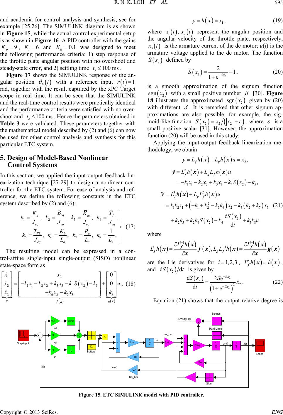

R. N. K. LOH ET AL. 595
ananalysis and synhesis, see for
exam ULINK diagrm is as n


1
y
h
d academia for control t
ple [25,26]. The SIM
Figure 15, while the act
a show
ental se
x

x. (19)
where




21 ,
x
txt represent the angular position and
the angular velocity of the throttle plate, respectively,


3
x
t is the armature current of the dc motor; u(t) is the
armature voltage applied to the dc motor. The function


2
S
x
defined by
in ual control experimtup
is as shown in Figure 16. A PID controller with the gains
9
p
K, 6
i
K and 0.1
d
K was designed to meet
the following performance criteria: 1) step response of
the throttle plate angular position with no overshoot and
steady-state error, and 2) settling time 100ms
s
t.
Figure 17 shows the SIMULINK response of the an-
gular position

Lt
 with a reference input


1rt

rad, together with the result captured b

2
2
21
1ex
Sx
 


, (20)
is a smooth approximation of the signum function


2
sgn
x
with a small positive number

[30]. Figure
18 illustrates the approximated 2

sgn

x
given by (20)
with different

. It is remarked that other signum ap-
proximations are also possible, for example, the sig-
moid-like function

 
222
xxxS


, where

is a
small positive scalar [31]. However, the approximation
function (20) will be used in this study.
y the xPC Target
ope in real time. It can be seen that the SIMULINK
and the real-time control results were practically identical
and the performance criteria were satisfied with no over-
shoot and 100ms
s
t. Hence the parameters obtained in
Table 3 were validated. These parameters together with
the mathematical model described by (2) and (6) can now
be used for other control analysis and synthesis for this
particular ETC system.
5. Design of Model-Based Nonlinear
Control Systems
sc
k lin-
ear con-
Applying the input-output feedback linearization me-
thodology, we obtain


2,
y
LhLhux 
fg
xx




2
112 233425
,
f
yLhLLhu
kxkxkxkS xk


 
gf
xx 
In this section, we applied the input-output feedbac
earization technique [27-29] to design a nonlin
troller for the ETC system. For ease of analysis and ref-
erence, we define the following constants in the ETC
system described by (2) and (6):






 
32
2
1211236 23 27 3
2
25 242438
d
d
ff
yLhLLh u
kk xkkkkxkkkx
Sx
kkkkS xkkku
t

 
 
g
xx

(21)
2341, , , ,
eq f
m
eq eq
sBT
KK
kkkk
JJ


567 8
1
, , , ,
eq eq
ba
eq a
PL
aa
JJ
KR
T
kkkk
JLLL







(17)
The resulting model can be expressed in a con-
trol-affine single-input single-output (SISO) nonlinear
state-space form
where


 


11
1
,
ii
ii
Lh Lh
LhLL h





ff
fgf
xx
xfxx
xx
gx
are the Lie derivatives for , 1, 2, 3i



o
Lh h
fxx,
and


2
dSxt
as
2
1122
1
2
0xx d is given by


 

3 32
6
4
27
5
383
0
x
kx kx
 
 
 






2
2e x
2
2
2
2
d
d1ex
Sx
x
kxkS xku
xkxkx
 

 

 


xgx
fx
k
, (18) t
 




. (22)
Equation (21) shows that the output relative degree is
Km_bar
Kb_bar

(t )

(t )

(t )
Ks*

(t )+Tpl
Ste p i npu t
Springs
Sign
Scope
Kp
9
Ki
6
Kd
0.1
1
s
1
s
1
s
1
s
Hard Limi t s
Tf
Beq
1/Jeq
0.4
Rt
0.4
1/La
du/dt
Battery
12
Ia
emf
Figure 15. ETC SIMULINK model with PID controller.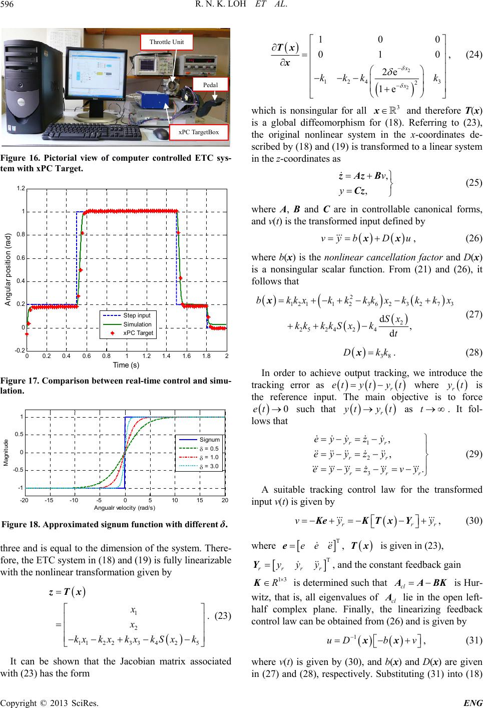

R. N. K. LOH ET AL. 596
Throttle Unit
xPC TargetBox
Peda l
Figure 16. Pictorial view of computer controlled ETC sys-
m with xPC Target. te
00.2 0.40.6 0.811.2 1.41.6 1.8 2
-0.2
0
0.2
0.4
0.6
0.8
1
1.2
Time
(
s
)
Angular p os iti on (rad)
Step i nput
Simulation
xPC Target
Figure 17. Comparison between real-time control and simu-
lation.
-20 -15 -10 -505 10 15 20
-1
-0.5
0
0. 5
1
Angual r vel oci t y (rad/ s)
Magni tude
Signum

= 0.5

= 1.0

= 3.0
Figure 18. Approximated signum function with different.δ
three and is equal to the dimension of the system. There-
fore, the ETC system in (18) and (19) is fully linearizable
with the nonlinear transformation given by
. (23)
It can be shown that the Jacobian matrix associated


1
2
11223 3425
x
x
kxkxkxkS xk







zTx
with (23) has the form


2
2
124 3
2
e
1e
10
01
2x
x
kkk k





0
0























Tx
x, (24)
which is nonsingular for all and therefore
T(x)
is a global diffeomorphism f. Referring to (23),
the original nonlinear system in the x-coordinates de-
scribed by (18) and (19) is transformed to a linear system
in the z-coordinates as
(25)
3
x
or (18)
,v

zB
,y Cz
where A, B and C are in controllable canonical forms,
and v(t) is the transformed input defined by
zA 


vybD u 
 xx, (26)
where b(x) is the nonlinear cancellation factor an
is a nonsingular scalar function. From (21) and (2
follows that
d D(x)
6), it




 
2
121126 227 333
k kxkkkkxkkkx
kk kkS


x
(27)
5422 4
2
2
d,
d
b
Sx
x kt 


38
Dkx.k
In order to achieve output tracking, we introduce the
tracking error as
(28)


r
etyty t

where


r
y
t
ective is to force
is
the reference input. The main obj


0et  such that


r
yt as t

ty

. It fol-
lows that
1,
rr
ez
e
yyy
yy
 







 
 2
3
,
.
rr
rr
z
eyy zy y
y
v


 



 



r
(29)
A suitable tracking control law for the transformed
r
y
input v(t) is given by

rr
vy



KeKTxY
 , (30)
where

T
eeee,


Tx is given in (23),

T
rrrr
yyy Y, and the constant feedback gain
13
R


K
is determined such that is Hur-
witz, that is, all eigenvalues of lie in the open left-
half complex plane. Finally, the linearizing fe
control law can be obtained from (26) and is given by
cl AABK
cl
A
edback


1
uDbv


 

xx,

(31)
whe
in
re v(t) is given by (30), and b(x) and D(x) are given
(27) and (28), respectively. Substituting (31) into (18)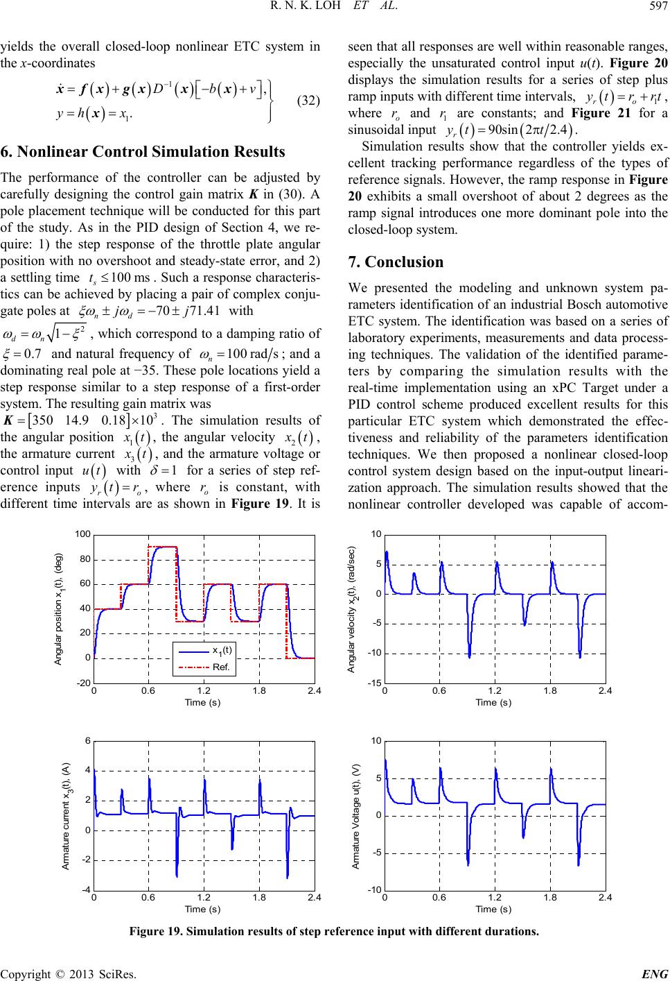

R. N. K. LOH ET AL. 597
yields the overall car ETC s in
the x-coordinates
 
 
losed-loop nonlineystem

 

1
1,
.
Dbv
yh x

 






x x
x
xfx gx
 (32)
6. Nonlinear Control Simulation R
The performance of the controller can be adjusted by
ca
que will be conducted for this part
of the study. As in the PID design of Sectio
quire: 1) the step response of the throttle pl
with no overshoot an and 2)
g time S
tics can be achju-
gate poles at
esults
refully designing the control gain matrix K in (30). A
pole placement techni
n 4, we re-
ate angular
positiond steady-state error,
a settlin0much a response characteris-10 s
s
t.
ieved by placing a pair of complex con
707
nd
jj1.41

  with
2
1
dn



, which correspoo a damping ratio of
0.7
nd t

 and natural frequency of 100 rads
n

; and a
dominating real pole at −35. These pole locations yield a
step response similar to a step response of a first-order
system. The resulting gain matrix was


3
350 14.90.1810K. The simulation results of
the angular position

1
x
t, the angular velocity


2
x
t,
the armature current


3
x
t, and the armature voltage or
control input


ut with 1

 for a series of step ref-
erence inputs

ro
y
tr, w
different time intervals are as sh
her
seen that all responses are well within reasonable ranges,
especially the unsaturated control input u(t). Figure 20
displays the simulation results for a series of step plus
ramp inputs with different time intervals,

1ro
y
trrt

,
where o and are constants; and Figure 21 for a
sinusoidal input
r1 r


90sin 22.4
r
yt t .
Simulation results show that the controller yields ex -
cellent tracking performance regardless of the types of
reference signals. However, the ramp response in Figure
20 exhibits a small overshoot of about 2 degrees as the
ramp signal introduces one more dominant pole into the
closed-loop system.
7. Conclusion
We presented the modeling and unknown system pa-
rameters identification of an industrial Bosch automotive
ETC system. The identification was based on a series of
laboratory experiments, measurements and data process-
ing techniques. The validation of the identified parame-
ters by comparing the simulation results with the
real-time implementation using an xPC Target under a
PID control scheme produced excellent results for this
particular ETC system which demonstrated the effec-
tiveness and reliability of the parameters identification
techniques. We then proposed a nonlinear closed-loop
control system design based on the input-output lineari-
zation approach. The simulation results showed that the
nonlinear controller developed was capable of accom-
e is constan
Figure 19
o
r
own in
t, with
. It is
00.6 1.2 1.8 2.4
-20
0
20
40
60
100
80
An gula r po sition x
1
(t)
Time (s)
, (deg)
x
1
(t)
Ref.
10
5
0
-5
-10
-1500.6 1.2
Angular velocity x
2
(t), (rad/ sec)
Tim e (s)1.8 2.4
610
00.6 1.2 1.8 2.4
-4
-2
0
2
4
A rma tu
Time (s)
re current x
3
(t), (A)
5
0
-5
-1000.6 1.2 1.8 2.4
Ar m ature Volta ge u(t) , (V )
Tim e (s)
ference input w i th diffe re nt dur ations. Figure 19. Simulation results of step re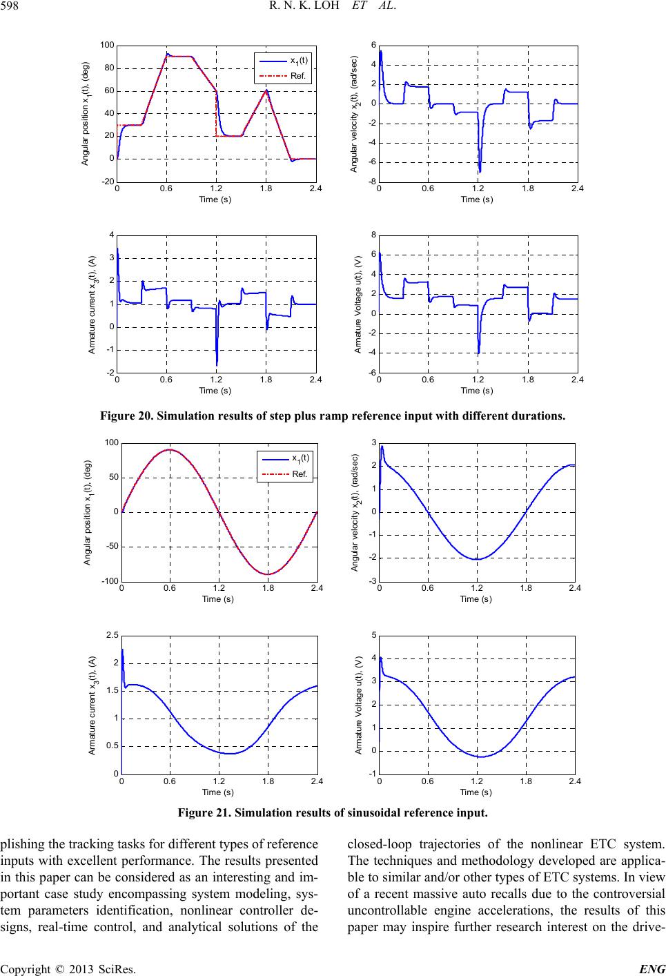

R. N. K. LOH ET AL. 598
00.6 1.2 1.8 2.4
-20
0
20
40
60
80
100
Angular position x
1
(t), (deg)
Time (s)
x
1
(t)
Ref.
00.6 1.2 1.8 2.4
-8
-6
-4
-2
0
2
4
6
Angular velocity x
2
(t), (rad/sec)
Time (s)
00.6 1.2 1.8 2.4
-2
-1
0
1
2
3
4
Arm ature current x
3
(t), (A)
Time (s)00.6 1.2 1.8 2.4
-6
-4
-2
0
2
4
6
8
Arm ature Voltage u(t), (V)
Time (s)
Figure 20. Simulation results of step plus ramp re ferenc e input with diffe re nt durations.
00.6 1.2 1.8 2. 4
-100
-50
0
50
100
An gu lar position x
1
(t ), (deg)
Time (s)
x
1
(t)
Ref.
3
2
00.6 1.2 1.8 2.4
-3
-2
-1
0
1
Angular velocity x
2
(t), ec)
Tim e (s)
(rad/s
2.5 5
00.6 1.2 1.8 2. 4
0
0. 5
1
1. 5
24
Armature current x
3
(t ), (A )
Time (s)
3
2
1
0
-100.6 1.2 1.8 2.4
A rmature V ol tage u(t ), (V )
Tim e (s)
Figure 21. Simulation results of sinusoidal refere nce input.
plishing the tracking tasks for different types of reference
inputs with excel
this paper can be considered as an interesting and im-
portant case study encompassing system modeling, sys-
tem parameters identification, nonlinear controller de-
signs, real-time control, and analytical solutions of the
closed-loop trajectories of the nonlinear ETC system.
d are applica-
ble to similar and/or other types of ETC systems. In view
of a recent massive auto recalls due to the controversial
uncontrollable engine accelerations, the results of this
paper may inspire further research interest on the drive-
lent performance. The results presented The techniques and methodology develope
in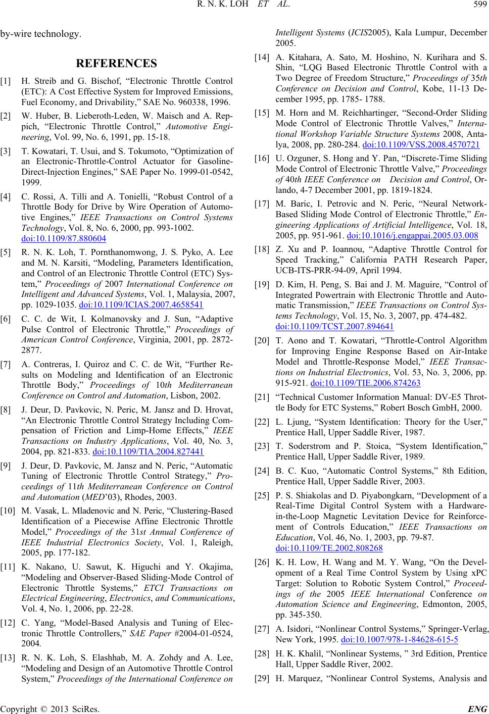

R. N. K. LOH ET AL. 599
by-wire technology.
REFERENCES
[1] H. Streib and G. Bischof, “Electronic Throttle Control
(ETC): A Cost Effective System for Improved Emissions,
Fuel Economy, and Drivability,” SAE No. 960338, 1996.
[2] W. Huber, B. Lieberoth-Leden, W. Maisch and A. Rep-
pich, “Electronic Throttle Control,” Automotive Engi-
neering, Vol. 99, No. 6, 1991, pp. 15-18.
[3] T. Kowatari, T. Usui, and S. Tokumoto, “Optimization of
an Electronic-Throttle-Control Actuator for Gasoline-
Direct-Injection Engines,” SAE Paper No. 1999-01-0542,
1999.
[4] C. Rossi, A. Tilli and A. Tonielli, “Robust Control of a
Throttle Body for Drive by Wire Operation of Automo-
tive Engines,” IEEE Transactions on Control Systems
Technology, Vol. 8, No. 6, 2000, pp. 993-1002.
doi:10.1109/87.880604
[5] R. N. K. Loh, T. Pornthanomwong, J. S. Pyko, A. Lee
and M. N. Karsiti, “Modeling, Parameters Identification,
and Control of an Electronic Throttle Control (ETC) Sys-
tem,” Proceedings of 2007 International Conference on
Intelligent and Advanced Syst
pp. 1029-1035. doi:10.1109/I
ems, Vol. 1, Malaysia, 2007,
CIAS.2007.4658541
[6] C. C. de Wit, I. Kolmanovsky and J. Sun, “Adaptive
Pulse Control of Electronic Throttle,” Proceedings of
American Control Conference, Virginia, 2001, pp. 2872-
2877.
[7] A. Contreras, I. Quiroz and C. C. de Wit, “Further Re-
sults on Modeling and Identification of an Electronic
Throttle Body,” Proceedings of 10th Mediterranean
Conference on Control and Automation, Lisbon, 2002.
[8] J. Deur, D. Pavkovic, N. Peric, M. Jansz and D. Hrovat,
“An Electronic Throttle Control Strategy Including Com-
pensation of Friction and Limp-Home Effects,” IEEE
Transactions on Industry Applications, Vol. 40, No. 3,
2004, pp. 821-833. doi:10.1109/TIA.2004.827441
[9] J. Deur, D. Pavkovic, M. Jansz and N. Peric, “Automatic
Tuning of Electronic Throttle Control Strategy,”
ceedings of 11th Mediterranean Conference on Control
and Automatio03.
ode Control of
g, “Model-Based Analysis and Tuning of Elec-
e Control
f the International Conference on
Intelligent Systems (ICIS2005), Kala Lumpur, December
2005.
[14] A. Kitahara, A. Sato, M. Hoshino, N. Kurihara and S.
Shin, “LQG Based Electronic Throttle Control with a
Two Degree of Freedom Structure,” Proceedings of 35th
Conference on Decision and Control, Kobe, 11-13 De-
cember 1995, pp. 1785- 1788.
[15] M. Horn and M. Reichhartinger, “Second-Order Sliding
Mode Control of Electronic Throttle Valves,” Interna-
tional Workshop Variable Structure Systems 2008, Anta-
lya, 2008, pp. 280-284. doi:10.1109/VSS.2008.4570721
[16] U. Ozguner, S. Hong and Y. Pan, “Discrete-Time Sliding
Mode Control of Electronic Throttle Valve,” Proceedings
of 40th IEEE Conference on Decision and Control, Or-
lando, 4-7 December 2001, pp. 1819-1824.
[17] M. Baric, I. Petrovic and N. Peric, “Neural Network-
Based Sliding Mode Control of Electronic Throttle,” En-
gineering Applications of Artificial Intelligence, Vol. 18,
2005, pp. 951-961. doi:10.1016/j.engappai.2005.03.008
[18] Z. Xu and P. Ioannou, “Adaptive Throttle Control for
Speed Tracking,” California PATH Research Paper,
UCB-ITS-PRR-94-09, April 1994.
[19] D. Kim, H. Peng, S. Bai and J. M. Maguire, “Control of
Electronic Throttle and Auto-
EE Transactions on Control Sys-
Pro-
n (MED’03), Rhodes, 20
[10] M. Vasak, L. Mladenovic and N. Peric, “Clustering-Based
Identification of a Piecewise Affine Electronic Throttle
Model,” Proceedings of the 31st Annual Conference of
IEEE Industrial Electronics Society, Vol. 1, Raleigh,
2005, pp. 177-182.
[11] K. Nakano, U. Sawut, K. Higuchi and Y. Okajima,
“Modeling and Observer-Based Sliding-M
Electronic Throttle Systems,” ETCI Transactions on
Electrical Engineering, Electronics, and Communications,
Vol. 4, No. 1, 2006, pp. 22-28.
[12] C. Yan
tronic Throttle Controllers,” SAE Paper #2004-01-0524,
2004.
[13] R. N. K. Loh, S. Elashhab, M. A. Zohdy and A. Lee,
“Modeling and Design of an Automotive Throttl
System,” Proceedings o
Integrated Powertrain with
matic Transmission,” IE
tems Technology, Vol. 15, No. 3, 2007, pp. 474-482.
doi:10.1109/TCST.2007.894641
[20] T. Aono and T. Kowatari, “Throttle-Control Algorithm
for Improving Engine Response Based on Air-Intake
Model and Throttle-Response Model,” IEEE Transac-
tions on Industrial Electronics, Vol. 53, No. 3, 2006, pp.
915-921. doi:10.1109/TIE.2006.874263
[21] “Technical Customer Information Manual: DV-E5 Throt-
tle Body for ETC Systems,” Robert Bosch GmbH, 2000.
[22] L. Ljung, “System Identification: Theory for the User,”
n,
ns on
Prentice Hall, Upper Saddle River, 1987.
[23] T. Soderstrom and P. Stoica, “System Identification,”
Prentice Hall, Upper Saddle River, 1989.
[24] B. C. Kuo, “Automatic Control Systems,” 8th Editio
Prentice Hall, Upper Saddle River, 2003.
[25] P. S. Shiakolas and D. Piyabongkarn, “Development of a
Real-Time Digital Control System with a Hardware-
in-the-Loop Magnetic Levitation Device for Reinforce-
ment of Controls Education,” IEEE Transactio
Education, Vol. 46, No. 1, 2003, pp. 79-87.
doi:10.1109/TE.2002.808268
[26] K. H. Low, H. Wang and M. Y. Wang, “On the Devel-
opment of a Real Time Control System by Using xPC
Target: Solution to Robotic System Control,” Proceed-
ings of the 2005 IEEE International Conference on
Automation Science and Engineering, Edmonton, 2005,
pp. 345-350.
[27] A. Isidori, “Nonlinear Control Systems,” Springer-Verlag,
New York, 1995. doi:10.1007/978-1-84628-615-5
[28] H. K. Khalil, “Nonlinear Systems, ” 3rd Edition, Prentice
Hall, Upper Saddle River, 2002.
[29] H. Marquez, “Nonlinear Control Systems, Analysis and

R. N. K. LOH ET AL. 600
Link Manipulators Using neural Networks,”
Mode Control
Design,” Wiley Interscience, Hoboken, 2003.
[30] H. A. Talebi, R. V. Patel and K. Khorasani, “Control of
Flexible-
Lecture Notes in Control and Information Sciences,
Springer-Verlag, London, 2001.
[31] C. Edwards and S. Spurgeon, “Sliding
Theory and Applicationsm” Taylor & Francis, London,
1998.