Open Journal of Acoustics
Vol.2 No.1(2012), Article ID:17795,9 pages DOI:10.4236/oja.2012.21003
Effect of Seabed Topography Change on Sound Ray Propagation—A Simulation Study
1Department of Scientific Research, Dalian Navy Academy, Dalian, China
2College of Physical and Environmental Oceanography, Ocean University of China, Qingdao, China
Email: 450344118@163.com
Received January 16, 2012; revised February 19, 2012; accepted February 29, 2012
Keywords: Sound Ray Propagation; Distance Correlation; Ray Model; Simulation
ABSTRACT
Variation of ocean environmental parameters is important to sound ray propagation. This article studies the problem of sound ray propagation in seawater by BELLHOP ray model. The sensitivities of sound ray propagation to the variations of seabed topography and depth of sound source by simulation. The results show that the depth variation of sound source is the main cause for emerging and disappearing of surface sound channel, accumulation area and deep sound channel. The deviation of sound ray propagation is in accordance with seabed topography change.
1. Introduction
When propagating in seawater, sound ray may be affected by environmental factors such as sea surface and submarine boundary. The study of sound ray propagation in seawater is mainly ray theory. Sound wave propagation in seawater is looked up as sound ray propagation in medium in the context of high frequency. The change of sound intensity, the time and distance of sound ray propagation in space are mainly studied. Ray acoustics is an approximate method, which is only for the sound wave of high frequency. But in many cases, this method is effective and effective to solve the problem in seawater [1].
Modeling and Simulating of sound wave propagation is important to sonar’s using and optimum designing in water. There are already some simulating study reports on sea sound propagation effect and characteristic of sound channel under perfect environment [2,3].
2. Numerical Model of Acoustic Propagation
To simulation study the difference of sound channel in different condition frames; it is emulational calculated the difference of sound channel by BELLHOP radial model. BELLHOP model by Gaussian approximate method, which was brought out by Porter, etc. [4], deals preferably with energy caustic and absolute shadow zone.
Supposing the sound pressure P on some sound ray propagation is:
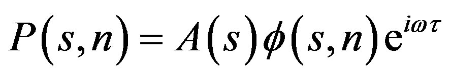 (1)
(1)
 is circumference ratio, A is amplitude on the direction of sound ray,
  is influence function which is perpendicular to the direction of sound ray, s is arc length on the direction of sound ray, n is displacement which is perpendicular to the direction of sound ray centre,
  is time of sound ray propagation.
In case of cylindrical coordinates, control equations of sound ray propagation are [5]:
 (2)
(2)
and r is horizontal distance, z is horizontal depth,  and
and  are two middle variables which have relationship of grazing angle,
  ,
, .
.
3. Simulation Calculation of Sound Ray Spreading Related with Distance
In BELLHOP model, supposing the sound velocity profile is like Figure 1, emulation calculated is under the condition of changing the environmental factors. When upslope, sound source is set as 50 m, 500 m, 1500 m and 4000 m under water; angle of incidence is 1˚, 3˚, 5˚, 8˚, respectively; frequency of sound wave is 1000 Hz; submarine substrate is silt, in accordance with the parameter of geoacoustics by Hamilton [6], substrate parameter: density is , compressional velocity is 1623 m/s, compressional attenuation coefficient is 0.673 dB/kHz; Y

Figure 1. Sound velocity profile.
is vertical depth, unit is meter (m), X is horizontal distance, unit is kilometer (km).
When downslope, case 1: sound source is set as 50 m under water, angle of incidence is 1˚, 3˚, 5˚, 8˚, respecttively, frequency of sound wave is 1000 Hz, submarine substrate is silt, Y is vertical depth, unit is meter (m), X is horizontal distance, unit is kilometer (km); case 2: sound source is set as 50 m under water, angle of incidence is –2˚, –1˚, 1˚, 2˚. Frequency of sound wave is 1000 Hz, submarine substrate is silt, Y is vertical depth, unit is meter (m), X is horizontal distance, and unit is kilometer (km).
When wavy terrain, case 1: sound source is set as 50 m, 500 m, 1500 m and 3000 m under water, angle of incidence is 1˚, 3˚, 5˚, 8˚, respectively, frequency of sound wave is 1000 Hz, submarine substrate is silt, Y is vertical depth, unit is meter (m), X is horizontal distance, unit is kilometer (km); case 2: sound source is set as 50 m under water, angle of incidence is –2˚, –1˚, 1˚, 2˚, Frequency of sound wave is 1000 Hz, submarine substrate is silt, Y is vertical depth, unit is meter (m), X is horizontal distance, and unit is kilometer (km).
4. Analysis of Simulation Result
Figure 1 is sound velocity profile. Figures 2-6, Figures 9-12 are the sound ray pictures of upslope and downslope under the conditions of different sound depths by emulation calculation. Figures 7-8 are the sound ray pictures of downslope under the conditions of two sound ray angles. Figure 9 and Figure 13 are the sound ray pictures of wavy terrain under the conditions of two sound ray angles.
4.1. The Influence of Submarine Topography
In picture, the distance of sound ray propagation is increasing as the horizontal distance increases in whole water area. The sound rays are convergence around the sound ray centre and sound ray bends to the sea bottom with biggish angle away from the center. The horizontal distances that the sound ray reaching sea bottom vary with different transmitting angles, and sound ray is emanative because of the different angles and horizontal distance increasing. Sound ray propagates in accumulation area form.

Figure 2. Ray picture for upslope seabed when setting sound source at 50 m below sea surface.

Figure 3. Ray picture for upslope seabed when setting sound source at 500 m below sea surface.
4.2. The Influence of Sound Velocity Profile
From Figures 2, 9 and 13, when sound source is set as 50 m, sound ray of specified angle propagates between 0 km and 50 km in horizon, surface channel appears between 0 m and 100 m in vertical, and surface channel turns to accumulation area when the distance increases in horizon. Because the sound velocity profile is constant speed structure in the depth of 100 m under seawater, surface channel emerges. In this channel, sound ray refracts so repeatedly that it loss huge energy and its velocity brings down. For this it could reach the sound velocity area of negative gradient, and propagates as accumulation area.
4.3. The Influence of Sound Source Depth
From Figures 2-6 and Figures 9-12, when sound source

Figure 4. Ray picture for upslope seabed when setting sound source at 1500 m below sea surface.

Figure 5. Ray picture for upslope seabed when setting sound source at 3000 m below sea surface.

Figure 6. Ray picture for upslope seabed when setting sound source at 4000 m below sea surface.

Figure 7. Ray picture for downslope seabed (case 1).

Figure 8. Ray picture for downslope seabed (case 2).

Figure 9. Ray picture for wavy terrain when setting sound source at 50 m below sea surface (case 1).

Figure 10. Ray picture for wavy terrain when setting sound source at 500 m below sea surface (case 1).

Figure 11. Ray picture for wavy terrain when setting sound source at 1500 m below sea surface (case 1).

Figure 12. Ray picture for wavy terrain when setting sound source at 3000 m below sea surface (case 1).

Figure 13. Ray picture for wavy terrain (case 2).
is set as different depth, sound ray propagates as different ways in those depths. 1) when sound source is set as 50 m under water, sound ray propagates 50 km in horizon as surface channel and accumulation area because of the sound velocity profile; 2) when sound source is set as 500 m under water, sound ray bends to the bottom, and refracts to the sea surface, then refracts to the bottom again. Because the phenomenon is iterative, it forms the accumulation area in wavy terrain and sound ray refracts iteratively in upslope; 3) when sound source is set as 1500 m under water in upslope, sound ray propagates between 500 m and 2500 m in vertical, and propagates with submarine topography; 4) when sound source is 3000 m under water, sound ray always bends to the general trends of sea surface, and refracts to the sea bottom, then refracts to the surface again. This phenomenon is iterative. Sound ray propagates with submarine topography when sound ray come under the topography just as upslope.
4.4. The Influence of Sound Ray Angle
When sound source is 50 m under water, sound ray of certain angles propagate as surface channel within sea surface. Case 1: when upslope and wavy terrain, angle of sound ray is . When the angle is
 , sound ray bends to sea surface as biggish angle, then refracts rapidly because of the biggish angle. Biggish angle makes sound ray in this angle range not refract in the speed boundary of constant speed structure, and can not propagate as surface channel; when the angle is
 , sound ray refracts in the speed boundary of constant speed structure instead of refraction, bends to the bottom instead of surface channel. Case 2: when downslope, sound ray propagates as surface channel in all angle, because sound rays of biggish angle bend to surface and bottom, form multiple refraction, original propagation angle are changed. This phenomenon makes sound ray propagate as sound channel.
1) when uoslope and wavy terrain, the angle is  , sound ray propagates as surface channel , propagation distance is increasing as
  increases (Figures 14 and 15). When
  increases 1˚, the propagation distance minish 2 - 3 km; 2) when sound ray comes under the downslope topography and propagates 50 km as surface channel in horizon (Figure 16) except the biggish angle. The distance of sound ray propagating minish erratically as angle
  increases; when the angle of sound ray refracting around sea surface is in agreement with topographical grade, sound ray refracts at sea bottom and propagates with topography, then separates from the bottom at 47 km in horizon as wave propagation instead of accumulation area (Figure 17).

Figure 14. Sound ray picture for upslope seabed.

Figure 15. Sound ray picture for downslope seabed with ray angles of 1˚, 3˚, 5˚, 8˚.

Figure 16. Sound ray picture for wavy terrain.

Figure 17. Sound ray picture for wavy terrain.
5. Conclusions
Ocean Environmental Factors has obviously regional and seasonal characteristic which are expressions of submarin topography’s undulation and the change of sound velocity profile. This article studies on the emulation of sound channel propagation in different conditions by HELLHOP radial model, discusses the sensitivity of sound ray propagation to the changes of these factors by changing submarin topography, depth of sound source and sound ray angle. Emulation calculation shows that:
1) it is more complicated on the influence by configuring of sound source—depth of receiving than the result of experience formula. When sound source is at 50 m, 500 m, 1500 m and 3000 m under water, it is influential on the propagation;
2) sound ray propagates with submarin topography, and the extent of pattern variation is similar to the extent of topographic pace;
3) sound ray angle is important to sound ray propagation. Sound ray propagates as surface channel within the distance of 50km in horizon. This distance is increasing as angle  minishs, and when
  increases 1˚, the propagation distance minishs 2 - 3 km.
REFERENCES
- B. s. Liu and J. y. Lei, “Hydroacoustics Theory,” 2nd Edition, Harbin Engineering University press, Harbin, 2010.
- J. Wang, J. g. Huang and J. Guan, “Wave Guide Modeling and Simulation for Underwater Acoustic Propagation,” Journal of System Simulation, Vol. 13, No. 1, 2001, pp. 37- 39.
- Y. z. Dong, X. m. Xu, P. x. Liu, et al., “Study on Modeling of Shallow Water Acoustic Channel and Its Applications,” Journal of System Simulation, Vol. 22, No. 1, 2010, pp. 47-55.
- M. B. Porter and H. P. Bucher, “Gaussian beam tracing for computing ocean acoustic fields,” Journal of the Acoustical Society of America, Vol. 82, No. 4, 1987, pp. 1349-1359. doi:10.1121/1.395269
- F. B. Jensen, W. A. Kuperman, M. B. Porter, et al., “Computational ocean acoustics,” American Institute of Physics Press, College Park, 1944.
- E. L. Hamilton, “Geoacoustic Modeling of the Sea Floor,” Journal of the Acoustical Society of America, Vol. 68, No. 5, 1980, pp. 1313-1340. doi:10.1121/1.385100