 Open Journal of Applied Sciences, 2012, 2, 115-121 doi:10.4236/ojapps.2012.22016 Published Online June 2012 (http://www.SciRP.org/journal/ojapps) Collocation Method for Nonlinear Volterra-Fr edholm Integral Equations Jafar Ahmadi Shali1, Parviz Darania2, Ali Asgar Jodayree Akbarfam1 1Department of Mathematics and Computer Science, University of Tabriz, Tabriz, Iran 2Department of Mathematics, Faculty of Science, Urmia University, Urmia, Iran Email: {j_ahmadishali, pdarania}@tabrizu.ac.ir, Akbarfam@yahoo.com Received April 18, 2012; revised May 14, 2012; accepted May 25, 2012 ABSTRACT A fully discrete version of a piecewise polynomial collocation method based on new collocation points, is constructed to solve nonlinear Volterra-Fredholm integral equations. In this paper, we obtain existence and uniqueness results and analyze the convergence properties of the collocation method when used to approximate smooth solutions of Volterra- Fredholm integral equations. Keywords: Collocation Method; Nonlinear Volterra-Fredholm Integral Equations; Convergence Analysis; Chelyshkov Polynomials 1. Introduction We shall consider the nonlinear Volterra-Fredholm inte- gral equation 12 ,0,ytgty tFy ttIT . (1) The Volterra integral operators given by 1 0 : ,, d, t CI CI tktsys s (2) where and and Fredholm integral operators given by 1 kCD ,:0Dts stT 2 0 : ,, d, T FCI CI ytktsys s (3) where ,1, rr2 kCII denotes (real or complex) parameters and and let be a given function. 2 IgC The mentioned equations are characterized by the presence of a linear functional argument and play an im- portant role in explaining many different phenomena. In particular, they turn out to be fundamental when or- dinary differential equations based model fail. These equations arise in industrial applications and in studies based on biology, economy, control and electro-dynamic. Collocation method is a widely popular numerical technique in solving integral equations, differential equa- tions, etc. When collocation method is used to solve complicated engineering problems, it has several disad- vantages, that is, low efficiency, ill-conditioned, etc. Thus, different types of techniques were proposed to improve the computational performance of collocation method. Recently, Chelyshkov has introduced sequences of polynomials in [1], which are orthogonal over the inter- val 0,1 with the weight function 1. These polynomials are explicitly defined by 1 0 1, mk jmkmkjk j mkjm k j Ptt km 0,1,,. (4) The polynomials mk Pt mk have properties, which are analogous to the properties of the classical orthogonal polynomials. These polynomials can also be connected to a fixed set of Jacobi polynomials . Precisely , m Pt 0,2 1 12 k k mk n k PttP t 1 . Investigating more on (4), we deduce that in the family of orthogonal polynomials have k multiple 0 mk m k Pt zeros 0t and mk distinct real zeros in the inter- val 0,1 . Hence, for every m the polynomial 0m Pt has exactly m simple roots in 0,1 . Following [1], it can be shown that the sequence of polynomials 00 mm Pt generate a family of orthogonal polynomials on 0,1 which possesses all the properties of other classic or- thogonal polynomials e.g. Legendre or Chebyshev poly- nomials. Therefore, if the roots of are chosen as collocation points, then we can obtain an accurate nu- merical quadrature. 0m Pt In the present paper, we further develop the works car- ried out in [2-6]. Copyright © 2012 SciRes. OJAppS  J. A. SHALI ET AL. 116 We discuss existence and uniqueness results and ana- lyze the convergence properties of the collocation method when used to approximate smooth solutions of linear Volterra-Fredholm integral equations and finally, some numerical results are presented in the final section, which support the theoretical results obtained in this paper. 2. Existence and Uniqueness Results Let denote the Banach space continuous real- valued functions, such that CI CI with max . tI g (5) Lemma 2.1. Assume H is a nonempty closed set in a Banach space V, and that is continuous. Suppose is a contraction for some positive integer m. Then, T has a unique fixed-point in H. :TH H m T Proof: For proof see [7]. Here, in integral Equation (1), we assume that for some constants i i k , satisfies a Lipschitz condition with respect to its third argument 121 ,, ,,, 0,,1,2. ii i i ktsyktsyMy y stT yi 2 (6) Theorem 2.2. Assume g and i satisfy the condition (6) and given functions k ,, i k are continuous on their domains. Moreover, assume 1 2. T (7) Then the integral Equation (1) has a unique solution .tIyC Proof: We define the nonlinear integral operator 12 :, , 0, TCI CI Ty tgty tFy t tI T (8) Let us show that for m sufficiently large, the operator is a contraction on . For m T CI 12 , yCI 12 11 12 0 21 22 0 ,,,, d ,,,,d t T Ty tTyt ktsys ktsyss ktsysktsyss (9) Then 12 112 0 21 2 0 1212 d d. . t T Ty tTytMysyss ysyss MtMTyy (10) Since 22 12 111 2 0 212 2 0 ,,,, d ,,,, d, t T Ty tTyt ktsTys ktsTyss ktsTysktsTyss (11) we get 2 2 1 22 12 212 . 2! Mt Ty tTytMTyy (12) By a mathematical induction, we obtain 12 1 212 . ! mm mm Tyt Tyt Mt MTy y m (13) Thus 12 1 212 . ! mm mm Tyt Tyt TM TMy y m (14) Since, 2 01TM then 2 lim 0, m mTM and 1 lim 0, ! m m M m the operator is a contraction on m T IC when m is chosen sufficiently large. By the Lemma 2.1, the operator T has a unique fixed-point in IC. 3. Collocation Method Let ,0,,1, n tnhn NtT N define a uniform partition for 0, ,TI and let 01 1 :0 , :, 01. NN nnn ttt T ttn N The mesh N is constrained in the following sense: T hN with a given mesh N we associate the set of its interior points, 1,,1n N:: Nn Zt . 1d For a fixed and, for given integers and the piecewise polynomial space 1N1,m dN md SZ is defined by ::;,01 n, Nm d md SZ uCIunN dd where πmd denotes the set of (real) polynomials of a degree not exceeding md . The dimension of this space is given by dim 1. Nm Nd d md SZ Copyright © 2012 SciRes. OJAppS  J. A. SHALI ET AL. 117 For integral equation, we have hence, the collocation space will be 1,d 1 1N m SZ . Let 1 1, N m n uSZ for all n t we have 1 , 0,1,,1 m nrn r ututshL sutch nN r (15) From (15) we see that an element 1 1, N m uSZ is well defined when we know the coefficients nr ut ch for all In order to compute these coef- ficients, we consider the set of collocation parameters 0, ,1.nN c : , where and define the set of collocation points by 1 0 m cc ,1 0 jn 1, 1. ,1, mN Nnj Xt ,:,1,,,0,, njn j ttchj mnN The collocation solution will be de- termined by imposing the condition that satisfies the integral Equation (1) on the finite set 1 1, mN uS Z u N 12 , , N utgtu tFut tX (16) Thus, for ,nj the collocation Equation (16) assumes the form n j ttt ch , ,,11, 0 22, 0 ,, d ,,d. nj t nj njnj T nj utgtk tsuss kt suss 17) From this equation and after some computations, we obtain 11 ,,11, 0 0 11, 0 11 22, 0 0 ,, ,,d ,,d j n njnjnj ii i c nj nn N nj ii i utgthktt shut shs hkttshutshs hkttshutshs d (18) Now, by using the local Lagrange basis functions 1 1, ,1,, mr rrl lr sc Lsl m cc , (19) for approximating the integral terms, we use the La- grange interpolating polynomial to approximate and , we obtain 1, ,, nj kt sus 2, ,, nj kt sus 1 , 11 ,11, 11 0 01 11, 1, 0 1 11 22,1 0 01 ,, ,,d ,,d. j nj nm njnj ii il mc nj nnljl l Nm nj iill il ut d thkttchutchLs hktt chut chLss hkttchu tchLss s ,, ,,m (20) Defining the quadrature weights 1 0 :d,1, ll wLssl m (21) and ,, 0 :d,,1, j c jl jl wLsslj (22) the fully discretized collocation equation corresponding to (20)-(22) is thus given by , 1 ,1 1, 01 1,1, 1 1 22, 01 ,, ,, ,,. nj nm njlnj ilil il m jln jnlnl l Nm lnjil il il ut thwktt chutch hwktt chut ch hwkttchutch (23) Note that, and Equation (23) represent for each 1 1 mN uS Z 0,1, ,1,nN a recursive system of m nonlinear algebraic equations with the unknowns ,nj ut . 4. Global Convergence Let denote the (exact) collocation solu- tion to (1) defined by (16). In our convergence analysis we examine the linear test equation 1 1 mN uS Z , 11 0 22 0 ,d ,d,0, t T ytgtktsyss ktsyss tIT (24) where 1,kCD 2.kCII We will assume that 1 2 is not in the spectrum of the Fredholm in- tegral operator F. A comment of the convergence results to the nonlinear Equation (1) can be found at the end of this section. Theorem 4.1. Assume that the given function in (24) satisfy 12 ,, mm m . CkC DkC II Then for all sufficiently small hTN the constrained mesh collo- cation solution to (24), for all 1 1 mN uS Z 1,N 0,1, ,n satisfies , m mm CMh (25) Copyright © 2012 SciRes. OJAppS  J. A. SHALI ET AL. 118 where m are positive constants not depending on h. This estimate holds for all collocation parameters C c with 1 Proof: In each interval 1ii, the exact solution y of (24) is m times continuously differentiable. This fol- lows from the smoothness hypotheses we have imposed on 12 01 m cc . tt ,, kk and from the expressions for t. From this it is obvious that both the left and right limits of t, as t tends to , exist and are finite. We will prove the estimate (25) by using the Peano’s Theorem to write nh , 1 , 0,1. mm nrnrmn r tshLsytchhR s s (26) Here, we have 1 ,0 :, m mn mn Rs Kszytzhz d, (27) and 1 1 1 1 ,, 1! 0,1 mm m mk k KszszLsc z m z k (28) Thus, it follows from (15) that the collocation error :yu possesses to the local representation ,, 1 ,(0,1 mm nrnrmn r tshLshRss ], (29) with and it satisfies the equation ,, njnjnj ytch utch , ,11, 0 22, 0 ,d ,d. nj t nj nj T nj tktss kt sss s (30) By substituting the (29) in the (30) and after some computations, we obtain 11 ,1 1, 0 01 11 1 11,, 0 0 11, 0 1 1 11,, 0 1 22, 0 ,d ,d ,d ,d ,d j j nm njnj irir ir n mnj imi i mc nj nrnr r c mnj nmn nj ir hkttshLss hkttshRss hkttshLss hkttshRss hkttshLss 1 01 11 1 22, , 0 0 ,d. Nm ir ir N mnj imi i hkttshRss (31) Define the matrices in , m L 1 1, 0 1, ,d , ,1,2,, 01 inj ir n kttshLss ij m inN , (32) 1, 0 2, ,d , ,1,2,, j c nj nr n kttshLss rjm (33) 1 2, 0 3, ,, ,1,2,, 01 inj ir n ktt shLsds rjm inN m , (34) and the vectors in by 1 1,1,, 0, 1,2,,,, T innjimi d, kttshRss jmi n (35) 2,1 ,, 0,d 1, 2,,, jT c nnjnmn , kttshRs s jm (36) 1 3,2 ,, 0,d 1, 2,,,, T innjimi , ktt shRss jmi n (37) ,1, 2,0,1,, T nnn nmnN 1, (38) by substituting the Equations (32)-(38) in Equation (31) we obtain 11 1 11,11,12, 00 11 11 12,23,23, 00 , nn ii m nninnn ii NN ii mm nni ii hhAh hAhh A n 1 , 0 N i i A (39) this linear algebraic system may be written more con- cisely as 1 12,23, 0 11 111 11, 11,12,23 00 Ni nnnni i nn ii mmm nin nn ii hh hhAhAh (40) Now, let 12,0 12,1 12,1 2B 00 02B 0 00 0 00 2B m m mN Ih Ih Ih (41) Copyright © 2012 SciRes. OJAppS  J. A. SHALI ET AL. 119 01 1 2 3,023,02 3,0 01 23,12 3,12 3,1 22 2 22 2 N m N NNm Ih hh Q hhIh (42) 1 N 0 1 1N 0i (43) Then we have 11 1 11,11, 0 1 11 12, 23, 0 22 22. nn ii m ni n i Ni mm nn i Qh hA hAh A (44) Since the kernel i is continuous on their domains, the elements of the matrixes 2, ,0,1,, nnN1 2,n h are all bounded. By using the Neumann Lemma the inverse of the matrix 1 2 nm I exists whenever 12, 1 2 n h for some matrix norm. This clearly holds whenever h is sufficiently small. In other words, there is an 0h so that for any mesh with ,hh each matrix n has a uniformly bounded inverse. Therefore, matrix has a uniformly bounded inverse. Also, the invertibility of the mm block matrix now depends not only on h but also on NN Q2 it is guar- anteed if 2 1, 2 F where * 2 2 0 :max, d, T tI 2 ktsskTk (45) assuming that 2 * 2 ,kts k and the elements of the matrixes Q are all bounded. Thus from (44), we get m In (46) where 1Q (47) and 11 1 11,11, 00 1 11 12,23, 0 22 +22. nn i m nni ii Ni mm n i hh hAh A 1 i n n A (48) It is clear that, matrix has a uniformly bounded in- verse and the elements of the matrixes are all bounded. Note that, from these assumptions and 11 ,Q there exists a constant so that for all mesh di- ameters 0 D 0, ,hh the uniform bound 1 0 1 , m P (49) holds. Here, for , m BL 1 (operator) norm induced by the -norm in Assume B denotes the matrix 1 l. m that 1 and 1, 1 1 in BP for 0 and 1,inN 1 2 1 From (46) and (48) we have .P 1 0 11 1 , mnn IP (50) 11 11 11, 11, 100 1 11 12,23, 01 111 01 101 1 0 11 2 112 22 22 22 , nn ii m nnin ii Ni mm nn i nm im i mm mm mm hhA hAh A PPhPhnmkM K hmkMKhNmkMK m (51) and hence 11 01 11 0 , nm im i Mh (52) where 0011101122 1, 12, 1 11 3, 2 1 11 11 00 [0,1] 2,21 ,, , ,,: , :max, d,:max,d. m inmmnmm im nmmm mm stI PP hPmK knNk AmkKMinAmkKM AmkKMinMy kKszzksvv k (53) Also, 1 1 1101 n mNm nj lj jlj (54) Then, from (52) and (54), we have 11 01 11 0 , 0,1,,1. nm nim i Mh nN Now, by using the discrete Gronwall inequality, we have 1 2 1, 0,1,,1, m nm Mh nN where exp .n 21 0 Now, by using the local error representation (29) this yields, setting :max , mj j WL 1, mm nmnmmm tshWhKM CMh m Copyright © 2012 SciRes. OJAppS 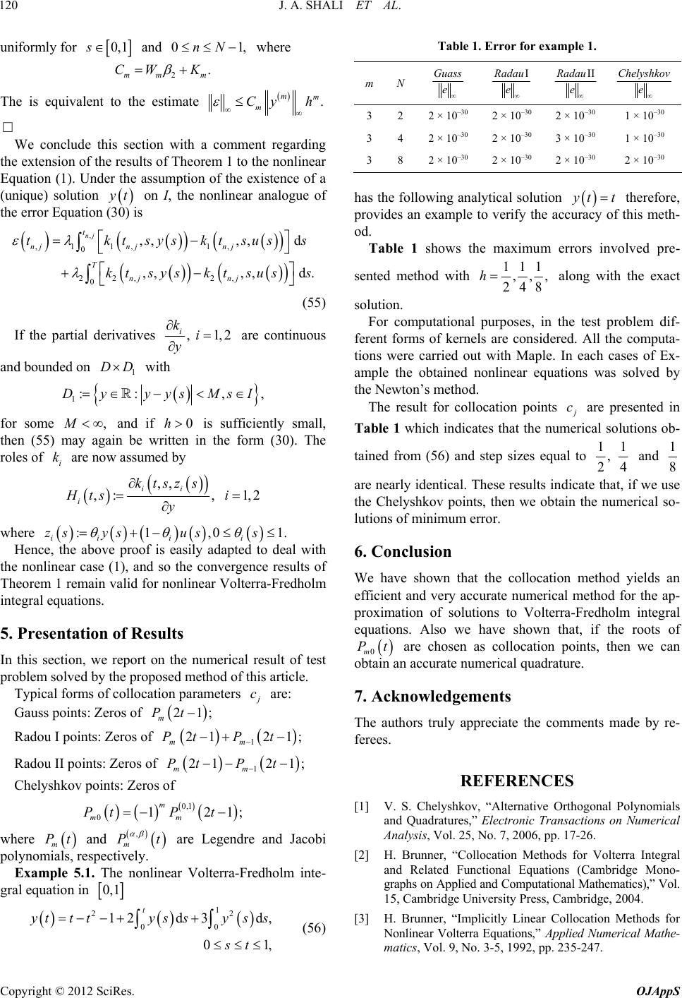 J. A. SHALI ET AL. 120 uniformly for 0, 1s and 01 where ,nN 2. mm m CW K The is equivalent to the estimate . mm m Cy h We conclude this section with a comment regarding the extension of the results of Theorem 1 to the nonlinear Equation (1). Under the assumption of the existence of a (unique) solution t on I, the nonlinear analogue of the error Equation (30) is , ,1 1,1, 0 22, 2, 0 ,,,, d ,,,, d. nj t nj njnj T nj nj tktsysktsus kt sysktsuss s (55) If the partial derivatives , 1,2 i ki y are continuous and bounded on with 1 DD 1:: ,Dy yysMsI , for some and if is sufficiently small, then (55) may again be written in the form (30). The roles of are now assumed by ,M i 0h k ,, ,:, 1,2 ii i ktszs Hts i y where :1,0 iiii zs ysuss 1. Hence, the above proof is easily adapted to deal with the nonlinear case (1), and so the convergence results of Theorem 1 remain valid for nonlinear Volterra-Fredholm integral equations. 5. Presentation of Results In this section, we report on the numerical result of test problem solved by the proposed method of this article. Typical forms of collocation parameters c are: Gauss points: Zeros of 21; m Pt Radou I points: Zeros of 1 21 21; mm PtP t 1; Radou II points: Zeros of 1 21 21; mm PtP t Chelyshkov points: Zeros of 0,1 012 m mm PtP t where and m Pt , m t are Legendre and Jacobi polynomials, respectively. Example 5.1. The nonlinear Volterra-Fredholm inte- gral equation in 0,1 1 2 00 12d3d, 01 t ytttys sys s st Table 1. Error for example 1. m N Guass e adau e adau e Chelyshkov e 3 2 2 × 10–30 2 × 10–30 2 × 10–30 1 × 10–30 3 4 2 × 10–30 2 × 10–30 3 × 10–30 1 × 10–30 3 8 2 × 10–30 2 × 10–30 2 × 10–30 2 × 10–30 has the following analytical solution tt therefore, provides an example to verify the accuracy of this meth- od. Table 1 shows the maximum errors involved pre- sented method with 111 ,,, 248 h along with the exact solution. For computational purposes, in the test problem dif- ferent forms of kernels are considered. All the computa- tions were carried out with Maple. In each cases of Ex- ample the obtained nonlinear equations was solved by the Newton’s method. The result for collocation points c are presented in Table 1 which indicates that the numerical solutions ob- tained from (56) and step sizes equal to 11 , 24 and 1 8 are nearly identical. These results indicate that, if we use the Chelyshkov points, then we obtain the numerical so- lutions of minimum error. 6. Conclusion We have shown that the collocation method yields an efficient and very accurate numerical method for the ap- proximation of solutions to Volterra-Fredholm integral equations. Also we have shown that, if the roots of 0m Pt are chosen as collocation points, then we can obtain an accurate numerical quadrature. 7. Acknowledgements The authors truly appreciate the comments made by re- ferees. REFERENCES [1] V. S. Chelyshkov, “Alternative Orthogonal Polynomials and Quadratures,” Electronic Transactions on Numerical Analysis, Vol. 25, No. 7, 2006, pp. 17-26. [2] H. Brunner, “Collocation Methods for Volterra Integral and Related Functional Equations (Cambridge Mono- graphs on Applied and Computational Mathematics),” Vol. 15, Cambridge University Press, Cambridge, 2004. 2 , (56) [3] H. Brunner, “Implicitly Linear Collocation Methods for Nonlinear Volterra Equations,” Applied Numerical Mathe- matics, Vol. 9, No. 3-5, 1992, pp. 235-247. Copyright © 2012 SciRes. OJAppS  J. A. SHALI ET AL. Copyright © 2012 SciRes. OJAppS 121 doi:10.1016/0168-9274(92)90018-9 [4] H. Brunner, “High-Order Collocation Methods for Sin- gular Volterra Functional Equations of Neutral Type,” Applied Numerical Mathematics, Vol. 57, No. 5-7, 2007, pp. 533-548. doi:10.1016/j.apnum.2006.07.006 [5] H. Brunner, “The Numerical Solution of Weakly Singular Volterra Functional Integro-Differential Equations with Variable Delays,” Communications on Pure and Applied Analysis, Vol. 5, No. 2, 2006, pp. 261-276. doi:10.3934/cpaa.2006.5.261 [6] A. T. Diogo, S. McKee and T. Tang, “A Hermite-Type Collocation Method for the Solution of an Integral Equa- tion with a Certain Weakly Singular Kernel,” IMA Jour- nal of Numerical Analysis, Vol. 11, No. 4, 1991, pp. 595- 605. doi:10.1093/imanum/11.4.595 [7] K. E. Atkinson and W. Han, “Theoretical Numerical Ana- lysis,” Springer, Berlin, 2009.
|