ABSTRACT

We establish, through solving semi-infinite programming problems, bounds on the probability of safely reaching a desired level of wealth on a finite horizon, when an investor starts with an optimal mean-variance financial investment strategy under a non-negative wealth restriction.

1. Introduction

In probability theory, the first passage-time problem is the study of the first moment when a stochastic process reaches a certain threshold. This problem often arises in financial mathematics and particularly in portfolio management. 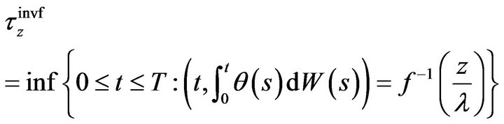For example, consider a risky strategy on an horizon [0,T], the investor may encounter a specific instant t when the amount of wealth be sufficient enough so that he may, at this point, safely reinvest all of his money in a simple bank account with (deterministic) interest rate and the resulting terminal wealth will attain his financial goal z. So we consider the following stopping time random variable :

(1)

and we naturally want to compute the probability

of such an event. If x₀ > 0 is his initial wealth then we will assume so that the investor cannot achieve his financial goal by simply placing his initial investment in a bank account.

2. Market Model

In order to investigate this goal-achieving problem, we must first define a mathematical setting for the dynamics of the financial market. We will consider here the celebrated Black-Scholes model that we next describe. The first asset is a bank account whose price at time t, , is the solution to the following ordinary differential equation (ODE):

(2)

The next assets consist of m stocks whose prices at time t are the solutions to the following SDEs (stochastic differential equations):

(3)

where is a standard m-dimensional Brownian motion.

We will assume that the interest rate r(t), stock appreciation rates b_i(t) and stock volatilities σ_ij(t) are deterministic functions and that

(4)

is invertible.

Let be a financial strategy (or portfolio) where is the amount placed in the i^th stock. If we assume that all strategies are self-financed (no outside injection of funds to the investors) and with no transaction costs then the wealth dynamic at time t is given by the following stochastic differential equation (SDE):

(5)

where.

Finally, among all the possible strategies, we will focus on the one generated by a family of stochastic control problems defined by

(6)

These are known as mean-variance problems and are considered the cornerstone of modern portfolio management theory which originated with the work of Nobel Prize laureate H. Markowitz.

3. Goal Achieving Probabilities

3.1. Case 1: Unconstrained and No Short-Selling Restriction

In this context, the optimal wealth process has the following form

(7)

with y₀ < 0, β > z and having specific values for the unconstrained and no-short selling (no borrowing stocks) case respectively. The computation of the probability, following a stochastic time change, can be reduced to the calculation of the probability of the first passage time of a Brownian motion with drift through a fixed level, more precisely the probability is given by:

(8)

where

(9)

is the cumulative density function of a standardized normal distribution.

Detailed proofs can be found in Li and Zhou [1] and Scott and Watier [2].

3.2. Case 2: No Bankruptcy Restriction

In this case, unfortunately, the optimal wealth process has a more complex expression, according to Bielecki et al. [3] it is given by

(10)

where

(11)

(12)

(13)

(14)

and and are Lagrange multipliers obtained by solving the nonlinear system of equations:

(15)

(16)

with

(17)

Evidently, an explicit form for the corresponding goalachieving probability 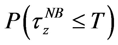as in the cases discussed in Section 3.1 appears unrealistic. However, we will show that we can obtain precise bounds for this probability through solving (deterministic) semi-infinite programming (SIP) problems.

The basic idea is to convert the original passage-time problem of this complex stochastic process with a fixed barrier into an equivalent passage-time problem for a simple Gaussian Markovian process but with a timevarying boundary.

To this end, the following result will be useful.

Let, then

(18)

is a strictly increasing function on the real line that takes on values in.

The proof is straightforward since clearly and, while

(19)

From this property we have that, for each fixed,

(20)

therefore, if

(21)

then

(22)

Due to the intricate nature of the time-varying boundary obtained, there is again little hope to find an explicit formula. But suppose we can get simpler boundaries h_l and h_u such that then clearly by defining

(23)

(24)

we would have

(25)

The next task at hand is to find suitable boundaries, for this, we need to recall first passage-time results for Gaussian Markovian processes through a specific family of time-varying boundaries known as Daniels’ curves (see Dinardo et al. [4]).

Consider the stochastic process

then the first passage-time probability through a boundary of the form

(26)

where

(27)

and, is given in explicit form by

(28)

Therefore the family of Daniels curves appears to be excellent candidates for obtaining explicit upper and lower bounds for our original goal-achieving problem. Finally, in order to generate the tightest bounds possible, we are naturally led to solve the following SIP problems:

(29)

and

(30)

For inquiries on efficient techniques for solving these SIP problems we refer the reader to Lopez and Still [5] and Reemtsen and Rückmann [6].

4. Numerical Examples

In order to illustrate that the solutions to the 3-parameter SIP problems can produce tight bounds, let us reprise the one stock market model example in Bielecki et al. that is but with different wealth objective z. Table 1 sums up the results.

Finally, we can easily show that the 80% rule (i.e., for all possible values of the market parameters) obtained by Li and Zhou and, Scott and Watier unfortunately does not hold in general for a nobankruptcy optimal mean-variance strategy. For example, if we set, by solving (29), we have .

5. Acknowledgements

The authors would like to thank the Editor and an anony-

mous referee for their helpful comments and suggestions. Grant Sponsor: Natural Sciences and Engineering Research Council of Canada.

REFERENCES

- X. Li and X. Y. Zhou, “Continuous-Time Mean-Variance Efficiency: The 80% Rule,” Annals of Applied Probability, Vol. 16, No. 4, 2006, pp. 1751-1763. doi:10.1214/105051606000000349
- A. Scott and F. Watier, “Goal Achieving Probabilities of Constrained Mean-Variance Strategies,” Statistics & Probability Letters, Vol. 81, No. 8, 2011, pp. 1021-1026. doi: 10.1016/j.spl.2011.02.023
- T. R. Bielecki, H. Jin, S. R. Pliska and X. Y. Zhou, “Continuous-Time Mean-Variance Portfolio Selection with Bankruptcy Prohibition,” Mathematical Finance, Vol. 15, No. 2, 2005, pp. 213-244. doi:10.1111/j.0960-1627.2005.00218.x
- E. Di Nardo, A. G. Nobile, E. Pirozzi and L. M. Ricciardi, “A Computational Approach to First-Passage-Time Problems for Gauss-Markov Processes,” Advances in Applied Probability, Vol. 33, No. 2, 2001, pp. 453-482. doi:10.1239/aap/999188324
- M. Lopez and G. Still, “Semi-Infinite Programming,” European Journal of Operational Research, Vol. 180, No. 2, 2007, pp. 491-518. doi:10.1016/j.ejor.2006.08.045
- R. Reemtsen and J.-J. Rückmann, “Semi-Infinite Programming,” Kluwer Academic Publishers, The Netherlands, 1998.