Energy and Power Engineering
Vol.10 No.09(2018), Article ID:87620,20 pages
10.4236/epe.2018.109026
Temperature Oscillations into a Couette-Poiseuille Flow
Shalom Sadik
Department of Mechanical Engineering, Ort Braude College, Karmiel, Israel

Copyright © 2018 by author and Scientific Research Publishing Inc.
This work is licensed under the Creative Commons Attribution International License (CC BY 4.0).
http://creativecommons.org/licenses/by/4.0/


Received: September 6, 2018; Accepted: September 26, 2018; Published: September 29, 2018
ABSTRACT
Following previous work that discussed temperature fluctuations without flowing media a physical model of temperature oscillations into a Couette-Poiseuille flow was built. The temperature distribution into the flow was calculated according to oscillations constraints on the upper and lower plates, and heat dissipation due to shear stresses into the fluid. The physical model deals with different temperature amplitudes and different frequencies constraints on the upper and the lower plates. A physical superposition and complex numbers were used. It was shown that when the constraint frequency increases, its penetration capacity is reduced. Increasing gap width between plates leads to increased fluid temperature values due to enlarged fluid velocity. Increasing thermal diffusivity, increases constrains temperatures penetration intensity.
Keywords:
Temperature, Amplitude, Frequency, Dissipation Function, Thermal Diffusivity

1. Introduction
The study of fluid flow in a Couette flow encompasses a few subjects as magneto hydrodynamics, porous media, particles suspension or two phases flow, and heat transfer in micro and nanoscale. These subjects applications relates for example to heat exchangers, heat pipes, electronic cooling, geophysics, biomedical instrumentation and gas flow at microscales. Several works relevant to these topics are cited below.
By using the Network Simulation Method (NSM), Beg et al. [1] examined the unsteady Hartmann-Coeutte flow and heat transfer in a parallel plate channel system containing a Darcian porous medium with lateral wall mass flux. The fluid was assumed as laminar, viscous and incompressible. Pressure gradient along the plates was assumed to be constant. Beg et al. work deals with some effects as Hall current, ion slip, viscous dissipation and Joule heating under a strong uniform transverse magnetic field. Constants values were determined for the temperatures boundary conditions on the upper and the lower plates. It was revealed that fluid temperature increased with increasing Darcy number (Da). Some conclusions: Increasing lateral wall mass flux-suction at the upper plate and injection at the lower plate decreased fluid principles velocities and temperature values. Increasing Hartmann number (Ha), which means stronger magnetic field, reduced primary velocity along the plates and increased secondary velocity due to Hall current, temperature value was reduced. Kuznetsov [2] performed an analytical solution to Couette flow in a composite channel, partially filled with a porous medium and partially with a clear fluid. The lower plate is moving and transfer constant heat flux, while the upper plate is fixed and adiabatic. It was shown that temperature value increases from the lower plate to the upper plate while the temperature gradient is decreases. Buonomo et al. [3] investigated fully developed, steady state forced convection in parallel-plate micro channels filled with a porous medium saturated with rarefied gases at high temperatures in local thermal non-equilibrium (LTNE) condition for the first-order slip-flow regime . A uniform heat flux was applied at both walls of the parallel-plate channel. The result showed that the internal dissipation increases as the velocity slip increases. Xu [4] investigated theoretically the thermal performance of multi-layered micro heat exchangers with porous media. It was shown that counter-flow heat exchanger is much more efficient than parallel-flow heat exchanger, and the micro heat exchanger with porous medium is preferable than the heat exchanger without a porous medium, especially for counter-flow heat exchanger. Makinde and Onyejekwe [5] investigated the steady flow and heat transfer of an electrically conducting fluid with variable viscosity and electrical conductivity between two parallel plates in the presence of a transverse magnetic field. It was assumed that couple of effects drove the flow: pressure gradient along the plates and upper plate constant velocity (the lower plate was fixed). The plates were kept at constant but different temperatures. The work showed that increasing the viscosity dependence at temperature caused the heat transfer rate to be reduced through the standing plate and increased through the moving plate. Hatami et al. [6] showed a study of magneto-hydrodynamic (MHD) Couette flows between two parallel infinite plates. The fluid between the plates was characterized as electrically conducting with particles suspension. The two phases: fluid phase and particle phase were tested. The upper plate was fixed and lower plate was time dependent. It was shown that when the magnetic field was fixed to the moving plate, increasing the intensity of the magnetic field (increasing Hartmann number) increases velocities of both phases, while the magnetic field was fixed to the standing plate, an inverse trend was received. Attia [7] investigated the MHD flow and heat transfer of a dusty and electrically conducting fluid in the presence of a uniform magnetic fluid while the variations of the viscosity and the electric conductivity of the fluid with temperature was taken under consideration. The governing equations were solved numerically using finite difference method. It was shown that increasing the fluid viscosity, increases the temperatures and velocities of the fluid and the dust particles. A similar investigation was performed by Eguia et al. [8] using network simulation method (NSM). Same results were received. Abd-Alla et al. [9] investigated the effect of both rotation and magnetic field of a micro polar fluid through a porous medium induced by sinusoidal peristaltic waves travelling down the channel walls. It was shown that the pressure gradient increases with increasing the rotation while it decreases with increasing the Hartmann number. It may be concluded that the rotation oppose the fluid flow while the magnetic field support the flow. Makinde and Chinyoka [10] investigated the unsteady flow and heat transfer of a dusty fluid between two parallel plates with variable viscosity and electric conductivity. The fluid was moving according to a constant pressure gradient while a magnetic field is acting perpendicular to the plates with Navier slip boundary condition. The plates were hold with constant but different temperatures. It was shown that increasing the slip intensity (parameter β) increases the velocities of both fluid and particles. There was not observed any temperatures variant of both fluid and particles by increasing slip intensity. Lockerby and Reese [11] introduced a study of steady-state micro Couette flow of a Maxwellian monatomic gas by applied Burnette equations. According to the results shown it may be concluded that maximum pressure distribution values is received for some intermediate Knudsen values, larger or lower Knudsen values leads to smaller pressure distribution values. A previous work under the same subject was performed by Xue et al. [12] . Comparative to Lockerby and Reese study it did not cover all Knudsen possible range. It was shown that the temperature distribution in slip flow is higher than that in non-slip flow.
The above works do not deal with the effect of temperature fluctuations on the two surfaces that surround the fluid in a Couette-Poisseuille flow on the fluid convection ability or on its ability to remove heat. The current work deals with oscillating temperature constraints on both plates. The temperature oscillations may be differ by amplitude and frequency. Heat dissipation due to shear stresses was taken under consideration. The current physical model was introduced as a function of dimensional parameters since it was wished to focus the results on truly parameters.
2. The Model Background
2.1. Couette-Poisseuille Flow
Couette-Poiseuille flow is a steady, one-dimensional flow between two plates with constant gap; the flow is along the plates or along the direction. Poiseuille flow structure and schematic velocity distribution is shown in Figure 1.
Poiseuille velocity distribution is parabolic and given as:
(1)
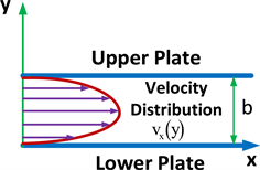
Figure 1. Poiseuille flow.
where is the velocity distribution along the axis, there is no velocity flow in the direction, is the dynamic viscosity, is the piezo metric pressure gradient, for horizontal plates the piezo metric pressure gradient is equal to the pure pressure gradient. More information about Couette-Poisseuille flow may be found for example in Fox et al. [13] .
2.2. The Energy Equation
The energy equation for a fluid is given as:
(2)
where is the fluid density, is the fluid specific capacity in a constant pressure, is the temperature material derivative, k is the fluid conductivity, is the temperature Laplacian, is the dynamic viscosity and is the dissipation function.
3. The Current Model
3.1. The Energy Model Equation
For Poiseuille flow, the dissipation value is received as:
(3)
(4)
The energy equation for two-dimensional coordinates is written as:
(5)
In Couette-Poiseuille flow there is no velocity component in the y direction, and there is no changes in the x direction, . The energy equation will be received as:
(6)
or as:
(7)
By marking:
(8)
and:
(9)
the energy equation will be received as:
(10)
or as:
(11)
by marking:
(12)
it is received that:
(13)
and:
(14)
With the energy equation will be received as:
(15)
According to the above definitions (Equation (12)), the following relations are received:
(16)
(17)
or:
(18)
Depending on only, the energy equation is received as:
(19)
or as:
(20)
Now, a new function is defined:
(21)
where the following relations are received:
(22)
(23)
(24)
(25)
(26)
Finally, the energy equation is received as:
(27)
or:
(28)
The last equation for oscillating solution is received (Sadik [14] ) as:
(29)
3.2. The Current Model―Basic Structure
The basic model structure is shown in Figure 2.
3.3. The Current Model―Stage 1
The first stage structure of the current model is shown in Figure 3.
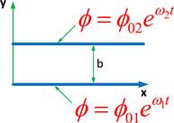
Figure 2. The current model―basic structure.

Figure 3. The current model―first structure.
The boundary conditions for this stage may written as:
(30)
The first boundary condition leads to the following relation:
(31)
or to:
(32)
The second boundary condition leads to the following connection:
(33)
or after dividing Equation (33) by it leads to:
(34)
It is received that:
(35)
By inserting value from Equation (32) into Equation (35), the following relations are received:
(36)
(37)
(38)
(39)
For this stage the first boundary condition may be written with its real value as , then related to the first boundary condition is received as , and related to T the first boundary condition is received as . With T the second boundary condition is received as .
In the initial time with at the boundaries it is received that and .
Full solution for is is and for , for T the full solution is received as .
For T, the initial condition is , or it may be written that .
3.4. The Current Model―Stage 2
The second stage structure of the current model is shown in Figure 4.
The boundary conditions for this stage may written as:
(40)
The first boundary condition leads to the following connections:
(41)
(42)
The second boundary condition leads to the following relations:
(43)
Equation (43) may be divided by to get:
(44)
(45)
(46)
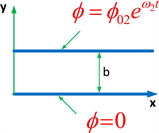
Figure 4. The current model second structure.
For this stage with T the first boundary condition is received as and the second boundary condition is received as .
In the initial time with at the boundaries it is received that and .
In a parallel way to the first stage, Full solution for is , for is and for T the full solution is received as .
For T, the initial condition is , or it may be written that .
3.5. The Current Model―Stage 3
Stage 3 is a simple addition of the results received at stage 1 and 2.
4. Results and Discussion
Figure 5 shows the functions and for intervals of 0.1667 s (1/6 s). The fluid characteristics were taken for air: specific capacity in constant pressure , dynamic viscosity , fluid density , thermal conductivity . Other parameters were taken as: , , . Every successive line from designate a progressive time interval of 0.1667 seconds. The phi and temperature plots are related to two time cycles. One time cycle is continued 1s , while two time cycles is continued 2 s. So, despite that in the phi plots, Figure 5(a), is introduced only six lines, actually it represent all the thirteen lines shown in Figure 5(b) ( , , , , , , , , , , , ). Figure 5(b) shows change of temperature over time. It is shown that fluid temperature increases with time progression compare to Figure 5(a) plots. Without heat dissipation the phi function would represent the temperature distribution as is shown in Figure 5(a). The temperature increasing in Figure 5(b) over the temperature area in Figure 5(a) is due to the dissipation function. All the plot lines in Figure 5 are symmetric related to the axis, according to identity of phi amplitudes and frequencies. What was written above can be shown clearly by following the black line in Figure 5(b) . The temperatures, which the black line represent, are highest according to maximum heat dissipation time. Its parallel line in the phi plot (Figure 5(a)) is the red line .This line can be considered as a reference line for the black line in Figure 5(b). Following the black line in Figure 5(b) shows maximum temperatures values near the plates where maximum shear stresses are produced and smaller temperature in the center according to extremum point area and smaller shear stresses.


Figure 5. and for intervals of 0.1667 s (1/6 s).
Figure 6 shows and for multiple distance between plates, other parameters are left unchanged. Figure 6(a) shows the limited penetration of the temperature constraints, the temperature absolute values in the middle area between plates are smaller than is shown in Figure 5(a). By comparing the black lines in Figure 5(b) and Figure 6(b) it is revealed that the temperature values in the middle area between plates in Figure 6(b) increases a little while near the plates the temperature values increases a lot. The fluid velocity between plates increases as a result of enlarged gap distance, this leads to increased pronounced shear stresses near the plates and significant heat dissipation in this area, where in the middle area the fluid velocities gradients are significantly smaller which leads to tiny temperature value increasing.
Figure 7 shows and for decreasing the upper phi amplitude to , other parameters remain unchanged according to Figure 5 as the basic figure. Figure 7 shows referring to both Figure 7(a) and Figure 7(b) the larger constraint amplitude penetration compare to the smaller amplitude penetration. By following every plot line, it may be concluded and seen that fluid temperatures follow the constraint temperature. By following for example the light blue line in Figure 7(a) it is shown that larger absolute temperatures values are received near the lower plate where the amplitude constraint is larger. By following the black line in Figure 7(b) where heat dissipation is also considered, the same diagnosis is shown, the temperature values near the lower plate are larger than the temperatures values near the upper plate.
Figure 8 shows and for decreasing absolute pressure gradient to 30 Pa/m (the real pressure gradient is −30 Pa/m in order to move the fluid in the direction, since the pressure gradient in the energy equation is in second power its real sign does not matter), other parameters remain unchanged according to Figure 5 as the basic figure. Since fluid velocity is strongly dependent on the pressure gradient, temperature rising is limited due to reduced shear stresses and heat dissipation. The black lines in Figure 5(b) and Figure 8(b) show clearly the contribution of the pressure gradient to heat dissipation and temperature rising, the absolute temperatures in Figure 5(b) where the absolute pressure gradient is larger have larger values than the temperatures in Figure 8(b) where the absolute pressure gradient is smaller. Figure 8 plots and what is written above referring to the pressure gradient is suitable for increasing four times the fluid dynamic viscosity.
Figure 9 shows and for increasing thermal conductivity to (the thermal diffusivity grows accordingly), other parameters remain unchanged according to Figure 5 as the basic figure. The increased thermal conductivity or the increased thermal diffusivity allows the heat to pass more easily into the fluid and follow the temperature constraints, it is shown clearly in both Figure 9 plots for and T. In order to follow the black line in Figure 9(b), the right border of the temperature value was increased to 40˚C. The increased temperatures into the fluid in Figure 9 which is


Figure 6. and for


Figure 7. and for


Figure 8. and for
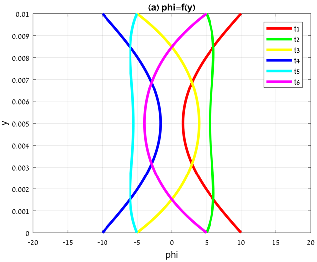
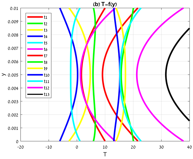
Figure 9. and for


Figure 10. and for

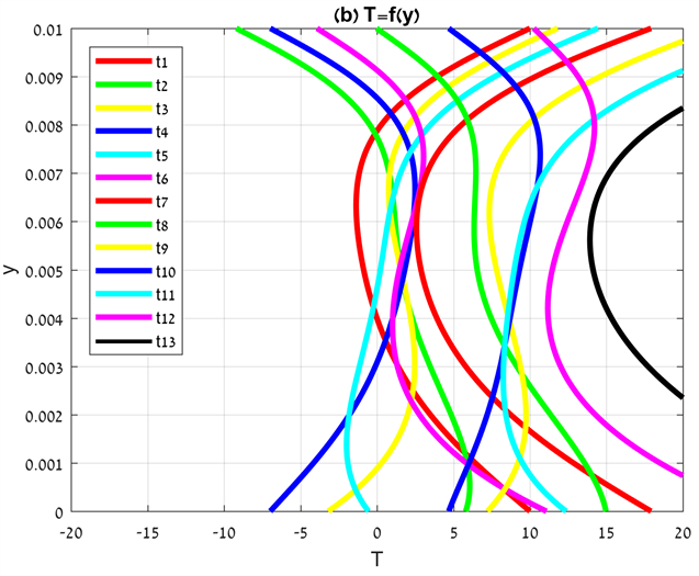
Figure 11. and for
greatly highlighted by the black line is due to the increased thermal conductivity or due to the increased thermal diffusivity and not to heat dissipation.
Figure 10 shows and for increasing two times the fluid density, to , other parameters remain unchanged according to Figure 5 as the basic figure. Changing the fluid parameters was performed only in order to examine the effect of those parameters; the changed parameters are not expected to characterize another real fluid. Increasing the fluid density leads to decreasing the thermal diffusivity and reduce the tracking ability of the fluid after the temperature constraints. This explanation is shown clearly in both plots of Figure 10 compare to the basic situation introduced in Figure 5. The same results and explanation are compatible for increasing two times the specific capacity, to 2014 J/kg∙K.
Figure 11 shows and for increasing upper constraint frequency to three times the lower constrain frequency, , other parameters remain unchanged according to Figure 5 as the basic figure. Both Figure 11 plots show the difference of the constraints intensity penetration to the fluid. It is shown in both Figure 11 plots that the temperatures values range near the upper plate with the larger frequency is smaller than the temperatures values range near the lower plate with the smaller frequency. Similar results for temperature fluctuations were obtained without a fluid media (Sadik [14] and [15] ). This result can be applied, for example, if it is necessary to remove heat by convection from an electronic chip that leads current with high frequency fluctuations or with high frequency of Ohmic power which causes to high temperature oscillations, and there is a limit on the convection liquid thickness, the thickness of the liquid needed may be reduced.
5. Conclusion
Main conclusion referred to the reduced penetration intensity of the enlarged frequency constraint. When the constraint frequency increases, its penetration capacity is reduced. Other conclusion relates to gap width between plates; larger gap width increases fluid temperatures due to fluid increased velocity. Referring to fluid thermal parameters, increasing thermal fluid conductivity or decreasing fluid density or decreasing heat specific capacity, increases constrains temperatures penetration intensity; this is due to enlarged thermal fluid diffusivity. Some expected results are shown: increasing gradient pressure leads to enlarged fluid velocity and more heat dissipation resulted in larger temperatures values into the fluid, increasing temperature constraint amplitude, and increasing heat penetration that leads to enlarged temperature into the fluid.
Declare
This work is dedicated to the memory of my mother and mother-in-law.
Conflicts of Interest
The author declares no conflicts of interest regarding the publication of this paper.
Cite this paper
Sadik, S. (2018) Temperature Oscillations into a Couette-Poiseuille Flow. Energy and Power Engineering, 10, 414-433. https://doi.org/10.4236/epe.2018.109026
References
- 1. Bég, O.A., Zueco, J. and Takhar, H.S. (2009) Unsteady Magnetohydrodynamic Hartmann-Coutte Flow and Heat Transfer in a Darcian Channel with Hall Current, Ionslip, Viscous and Joule Heating Effects: Network Numerical Solutions. Communications in Nonlinear Science and Numerical Simulation, 14, 1082-1097. https://doi.org/10.1016/j.cnsns.2008.03.015
- 2. Kuznetsov, A.V. (1998) Analytical Investigation of Couette Flow in a Composite Channel Partially Filled with a Porous Medium and Partially with a Clear Fluid. International Journal of Heat and Mass Transfer, 41, 2556-2560. https://doi.org/10.1016/S0017-9310(97)00296-2
- 3. Buonomo, B., Manca, O. and Lauriat, G. (2016) Forced Convection in Porous Microchannels with Viscous Dissipation in Local Thermal Non-Equilibrium Conditions. International communications in Heat and Mass Transfer, 76, 46-54.
- 4. Xu, H. (2017) Performance Evaluation of Multi-Layered Porous-Medium Micro Heat Exchangers with Effects of Slip Condition and Thermal Non-Equilibrium. Applied Thermal Engineering, 116, 516-517. https://doi.org/10.1016/j.applthermaleng.2016.12.090
- 5. Makinde, O.D. and Onyejekwe, O.O. (2011) A Numerical Study of MHD Generalized Couette Flow and Heat Transfer with Variable Viscosity and Electrical Conductivity. Journal of Magnetism and Magnetic Materials, 323, 2757-2763. https://doi.org/10.1016/j.jmmm.2011.05.040
- 6. Hatami, M., Hosseinzadeh, K., Domairry, G. and Behnamfar, M.T. (2014) Numerical Study of MHD Two-Phase Couette Flow Analysis for Fluid-Particle Suspension between Moving Parallel Plates. Journal of the Taiwan Institute of Chemical Engineers, 45, 2238-2245. https://doi.org/10.1016/j.jtice.2014.05.018
- 7. Attia, H.A. (2006) Unsteady MHD Couette Flow and Heat Transfer of Dusty Fluid with Variable Physical Properties. Applied Mathematics and Computation, 177, 308-318. https://doi.org/10.1016/j.amc.2005.11.010
- 8. Eguía, P., Zueco, J., Granada, E. and Patino, D. (2011) NSM Solution for Unsteady MHD Couette Flow of a Dusty Conducting Fluid with Variable Viscosity and Electric Conductivity. Applied Mathematical Modeling, 35, 303-316. https://doi.org/10.1016/j.apm.2010.06.005
- 9. Abd-Alla, A.M., Abo-Dahab, S.M. and Al-Simery, R.D. (2013) Effect of Rotation on Peristaltic Flow of Micropolar Fluid through a Porous Medium with an External Magnetic Field. Journal of Magnetism and Magnetic Materials, 348, 33-43. https://doi.org/10.1016/j.jmmm.2013.06.030
- 10. Makinde, O.D. and Chinyoka, T. (2010) MHD Transient Flows and Heat Transfer of Dusty Fluid in a Channel with Variable Physical Properties and Navier Slip Condition. Computers and Mathematics with Applications, 60, 660-669. https://doi.org/10.1016/j.camwa.2010.05.014
- 11. Lockerby, D.A. and Reese, J.M. (2003) High-Resolution Burnett Simulations of Micro Couette Flow and Heat Transfer. Journal of Computational Physics, 188, 333-347. https://doi.org/10.1016/S0021-9991(03)00162-1
- 12. Xue, H., Ji, H.M. and Shu, C. (2001) Analysis of Micro-Couette Flow Using Burnett Equations. International Journal of Heat and Mass Transfer, 44, 4139-4146. https://doi.org/10.1016/S0017-9310(01)00062-X
- 13. Fox, R.W., McDonald, A.T., Pritchard, P.J. and Leylegian, J.C. (2012) Fluid Mechanics. 8th Edition, John Wiley & Sons, Hoboken.
- 14. Sadik, S. (2018) A Three-Layers Plane Wall Exposed to Oscillating Temperatures with Different Amplitudes and Frequencies. Energy and Power Engineering, 10, 165-185. https://doi.org/10.4236/epe.2018.104012
- 15. Sadik, S. (2017) A Model of Two Cylindrical Plane Wall Exposed to Oscillating Temperatures with Different Amplitudes and Frequencies. Journal of Zhejiang University-SCIENCE A, 18, 974-983.