Received 4 June 2015; accepted 3 April 2016; published 6 April 2016

ABSTRACT

A simple methodology was shown in order to determine when a lonely star of a certain type might have a planetary family like the one of the Sun’s.

Keywords:

Planetary Systems Similar to the Solar System

1. Introduction

The Solar system is unique in the Universe in the sense that we do not know any other star which has planets revolving about it, and resembling those of the Sun’s family. It is important to detail the very special structure that the Solar system has.

The Solar system consists of the Sun and a large number of smaller objects gravitationally associated with it. These other objects are the planets, their satellites, the asteroids or minor planets, the comets, the meteoroids, and an interplanetary medium of very sparse gas and microscopic solid particles. Differently from the Sun, the planets are small, relatively cool, and five of them are solid. They give off no light of their own but shine only by reflected sunlight [1] .

The four innermost planets are Mercury, Venus, Earth, and Mars, and also they are called Inner planets. The four largest planets are gaseous and often are called the Jovian planets; and the others, including Pluto, are the Terrestrial planets [1] . On the other hand, we find that only the planets Venus, Earth, and Mars, and possibly Europa, one of Jupiter’s moons, possess conditions under which we can imagine forms of living organisms to exist. Of these four possibilities, only Earth offers conditions compatible with the existence of higher forms of plant or animal life as we know them [1] . It is often pointed out that the Sun is a typical star, and there must be many other stars with planetary systems similar to that of the Sun’s. Regarding the Sun, it is known that it is a yellow dwarf of a fifth-magnitude star [1] . It has a mean rotation period of 26.5 days but, as Carrington discovered, its surface rotates differentially; the polar rotation period is about 35 days [2] .

Between 1911 and 1913, the astronomers E. Hertzsprung and H. N. Russell, led independently to an extremely important discovery concerning the relation between the luminosities and surface temperatures of stars. The discovery is exhibited graphically on a diagram named in honor of the two Scientists, the Hertzsprung-Russell or H-R diagram [1] [3] . Two easily derived characteristics of stars of known distances are their absolute magnitudes or luminosities and their effective temperatures. The absolute magnitudes can be found from the known distances and the observed apparent magnitudes. The effective temperature of a star is indicated either by its color or its spectral class [1] [3] .

The most significant feature of the H-R diagram is that the stars are not distributed over it at random, exhibiting all combinations of absolute magnitude and temperature, but rather cluster into certain parts of the diagram. The majority of stars are aligned along a narrow sequence running from the upper left of hot, highly luminous part of the diagram to the lower right of cool, less luminous part. This band of points is called the Main Sequence [1] - [3] . A substantial number of stars lie above the Main Sequence on the H-R diagram in the upper right of cool, high luminosity region. These are called giants. At the top part of the diagram are stars of even higher luminosity, called supergiants. There are stars in the lower left of hot, low luminosity corner known as white dwarfs [1] - [3] . To say that a star lies on, or off the Main Sequence does not refer to its position in space, but only to the point that represents its luminosity and effective temperature on the H-R diagram [1] - [3] . It is estimated that about 90 percent of the stars in our part of space are Main-Sequence stars and about 10 percent are white dwarfs. Less than 1 percent is giants or supergiants [1] [3] . The Sun is a Main-Sequence star.

In order to give a solution to the problem of identifying stars which possess planetary systems similar to the Solar System all the binary and multiple systems, must be discarded from the set of Main-Sequence stars, only focusing the attention on lonely stars; in such a way that the problem is reduced to localize lonely yellow dwarfs, of slow rotation, and of dimensions and basic characteristics similar to those of the Sun’s (see Appendix).

2. Theoretical Methodology to Calculate the Basic Parameters of Any Gaseous Star

In the specialized literature [1] [4] , it is shown that knowing both the spectral class and luminosity class, a star’s position on the H-R diagram is uniquely determined [1] [3] [4] ; such that its absolute magnitude therefore is also known, and its distance can be calculated [1] [3] [4] .

As will be seen next, the values of the main parameters of any gaseous star can be obtained by direct calculation with only two observational data, such as the effective temperature and the absolute magnitude [5] .

The radius of any gaseous star can be calculated from those observational data, and using the magnitude of the self-generated magnetic field at the surface of the star [6] . It can be shown that the absolute value of that magnetic field is as follows [5] [6]

(1)

where T_e is the effective temperature, the subscript s indicates the surface, and

(2)

is a universal constant [5] [6] , with a the constant of Stefan’s law [5] [6] .

On the other hand, from the well known relationships [3] [5] [7]

(3)

and

(4)

where L is the luminosity, c the velocity of light in the empty space, M_bol the bolometric or absolute magnitude, and the symbol ¤ indicates the Sun, considering it as the unit of measure [7] . Substituting (3) in (4) and taking (1) into account it is obtained by direct calculation the following expression to obtain the stellar radius

(5)

Then the luminosity can be easily calculated from the relationship (3) using the value of the effective temperature.

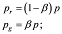
In order to determine the mass of any gaseous star, it is first necessary to calculate the value of the b parameter for such star. This parameter is defined as follows [3] [4] [8]

(6)

where p_r(x, t) is the pressure from the radiation, p_g(x, t) is the pressure from the hot gases and p(x, t) is the total pressure. From the modified mass-luminosity relationship [8]

(7)

where G is the gravitational constant, M is the stellar mass, k_c is the opacity coefficient which for numerical calculations is customary to assume that k_c = k , and a = 2.5 is a constant indicating an intense and uniform concentration of energy generating sources at the center of the star [3] , and from the following equations

(8)

which is the commonly accepted law for radiation absorption [3] . Furthermore, from the following relationship

(9)

Which is a formula that can be used to calculate the temperature at the center of the star [3] [8] ; and finally, also from the following relationship obtained from the theory of the polytropic gas sphere [3] [9] which also is used as another alternative formula to calculate the temperature at the center of the star

(10)

it is obtained the following [5]

(11)

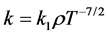
In these last equations, r(x, t) is the mass density, and T the temperature both that the center of the star, R is the gas constant, m is the average molecular weight whose numerical value is almost always taken equal to 2.11 [5] , k₁ is a constant, n is a positive integer number, and M´ = 2.015, and R’ = 6.901 [3] . It can be shown that for gaseous stars n = 3 [3] , in such a way that from (11) the following expression

(12)

is obtained [5] . Here the following relationship [3] [6]

(13)

was used to obtain the following formula [5]

(14)

in order to eliminate from 85,299.20-(11) the mass M.

With the numerical values of the constants (see Appendix) substituted in (12) the following result, which is valid for any gaseous star [6] , can be obtained

(15)

According to the previous statement, any two stars can be compared if one of them is considered as the appropriate unit of measure. It is common practice to use the brightest component of Capella binary system [6] ; for which the numerical values of its basic parameters are known. Consequently from Equation (15) the following formula can be obtained

(16)

where the asterisk refers to the particular star which is being compared to Capella. With the numerical data for this last star (see Appendix) one gets [5]

such that in (16) the following is obtained

(17)

Since the effective temperature is a conventional measure used to specify the flow of radiant heat emitted per unit area by any gaseous star [3] [6] , it can be shown that for gaseous stars, the constants k₁ and k₁ appearing in equation(17), keep the same proportion among themselves as that of their respective effective temperatures [5] . In such case, the ratios k₁/k₁ and T_e/T_e are numerically equal, such that it is always true that [5]

(18)

For any couple of gaseous stars which can be compared between themselves [5] . Consequently, from relationship (17) the following numerical equation for the calculation of b parameter for any gaseous star is obtained [5]

(19)

where

(20)

is a constant for each particular star under study. For the solution of numerical equations, Newton’s method is used [10] .

Once the parameter b has been obtained, the following fourth degree equation is used to determine the mass of the star [1] [2] ; considering that m = 2.11 [3] [5] [6]

(21)

In this way, one gets all the necessary results to calculate the volume, and the average mass density. The central mass density is obtained from the following formula from the theory of the polytropic gas sphere [3] [6]

(22)

where the subscripts indicates the central and the average mass density, respectively.

With the former method, the opacity coefficient, the temperature at the center of the star, and the magnitude of the self-generated magnetic field at any point inside the star can also be estimated [5] . The distance at which the star is found can be calculated using the visual and bolometric magnitudes in the following expression [1] [5]

(23)

where r_* is the distance in parsecs.

3. Solar and Stellar Rotation

Galileo first demonstrated that the Sun rotates on its axis when he observed the apparent motions of the Suns pots across the solardish [1] . Lastly, in 1859 R. Carrington found that the Sunrotated differentially [2] in such a way that the equatorial rotation period being about 25 days, while at high latitudes the period is about 35 days [2] . The Sun’s rotation rate can be determined also from the difference in the Doppler shifts of the light coming from the receding and approaching limbs. The solar rotation determined from the Doppler method confirms that the Sun rotates most rapidly at low latitudes, and with a longer period at high latitudes. At a latitude of 75˚, the rotation period is about 33 days, and at the poles it may be nearly 35 days. Its direction of rotation is from west to east [1] [2] . If a star is rotating, unless it axis of rotation happens to be directed toward the Sun, one of its limbs approaches us, and the other recedes from us, relative to the star as a whole. A star, however, appears as a point of light, and we are forced to analyze the light from its entire disk at once. Nevertheless, if the star is rotating, part of the light from it, including the spectral lines is shifted to shorter wavelengths and part is shifted to longer wavelengths. Each spectral line of the star is a composite of spectral lines originating from different parts of the star´s disk, all of which are moving at different speeds with respect to the observer. The effect produced is that all its spectral lines are broadened so that their profiles have a characteristic dish shape [1] . Fortunately, this dish shape is highly characteristic and usually can be distinguished from broadening produced by other sources [1] . The amount of rotational broadening of the spectral lines, if observable, can be measured, and a lower limit to the rate of rotation of the star can be calculated [1] .

The exact formula for the Doppler shift is

(24)

wherel is the wavelength emitted by the star, Dl is the difference between l and the wavelength measured by the observer, c is again the velocity of light in the empty space, and v is the relative line of sight velocity of the observer and the star, which is counted as positive if the velocity is one of recession and negative if it is one of approach [1] . If the relative line of sight velocity of the star and the observer is small compared to the velocity of light, however, the Equation (24) reduces to the following simple form, which is normally used [1]

(25)

On the other hand, for a gaseous star, it is always true that [3] [5] [8]

(26)

where E is the energy density radiated by the star considered as a black body [6] . The former equation is Stefan’s law [3] [6] . Now, E_V is the total energy E_T radiated by the star as thermal radiation. On the other hand, it is

easy to see that E_T =; where n is the number of photons with wavelength l in the volume V, and E_l the energy of each photon. Thus,

(27)

where n/V is the density of thermal radiation, and the Equation (26) was used. Moreover, and according to Planck’s equation

(28)

with h Planck’s constant [3] [6] . Hence, comparing (27) and (28) one gets that

(29)

Substituting (29) in (26) the following result valid for any gaseous star is obtained

(30)

In this case, any gaseous star can be compared with the Sun to obtain the following relationship

(31)

Nevertheless, it is easy to see that in (31) the term corresponding to the one of the effective temperatures is the dominant; so that it can be assumed that Dl_* » Dl to finally obtain as a good approximation that

(32)

where the numerical values of and were used. With this last relationship, the theoretical scheme to identify if a lonely star can have a planetary family similar to that of the Sun’s is completed.

4. Conclusion

With the help from the theoretical methodology presented, it is proposed the configuration of an observational program over the Main-Sequence stars, which consists of a systematical search of lonely yellow dwarfs, whose basic parameter is similar to those of the Sun’s; in order to obtain a group of stars which have high probability to possess a planetary family of the solar type, and where in some of those systems may be likely the natural conditions for forms of living organisms exist.

Cite this paper

Angel Fierros Palacios, (2016) The Problem of the Existence of Planetary Systems Similar to the Solar System. Journal of High Energy Physics, Gravitation and Cosmology,02,161-167. doi: 10.4236/jhepgc.2016.22015

References

Appendix

References

- 1. Adell, G. (1964) Exploration of the Universe. Holt, Rinehart and Winston. New York, Chicago.
- 2. Wilson, P.R. (1994) Solar and Stellar Activity Cycles. Cambridge Astrophysics Series: 24. Cambridge University Press, New York. http://dx.doi.org/10.1017/CBO9780511564833
- 3. Eddington, A.S. (1988) The Internal Constitution of the Stars. Cambridge University Press, New York. http://dx.doi.org/10.1017/cbo9780511600005
- 4. Palacios, A.F. (2004) The Hamilton-Type Principle in Fluid Dynamics. Fundamentals and Applications to Magnetohydrodynamics, Thermodynamics, and Astrophysics. Springer-Verlag, Wien, New York.
- 5. Palacios, A.F. (2003) The Effective Temperature and the Absolute Magnitude of the Stars. To Be Publishing.
- 6. Wehr, M.R. and Richards, J.A. (1960) Physics of the Atom. Addison-Wesley Publishing Co., Reading, London.
- 7. Shwarzchild, M. (1965) Structure and Evolution of the Stars. Dover Publications Inc., New York.
- 8. Palacios, A.F. (2003) The Magnetic Field in the Stability of the Stars. To Be Publishing.
- 9. Emden, R. (1907) Gaskugeln: Anwendugen der Mechanischen Warmetheoric. B.G. Tewbner, Leipzig and Berlin.
- 10. Leonard, E.D. (1964) New First Course in the Theory of Equations. John Wiley & Sons, Inc., New York.