Open Journal of Biophysics
Vol. 2 No. 4 (2012) , Article ID: 24107 , 4 pages DOI:10.4236/ojbiphy.2012.24015
Simplifying the Analysis of Enzyme Kinetics of Cytochrome c Oxidase by the Lambert-W Function
1Department of Molecular Spectroscopy, Max Planck Institute for Polymer Research, Mainz, Germany
2Department of Physics, Experimental Molecular Biophysics, Freie Universitaet Berlin, Berlin, Germany
3Department of Chemistry, Physical and Biophysical Chemistry, Bielefeld University, Bielefeld, Germany
Email: schleeger@mpip-mainz.mpg.de, jheberle@zedat.fu-berlin.de, sergej.kakorin@uni-bielefeld.de
Received June 6, 2012; revised July 20, 2012; accepted August 10, 2012
Keywords: Cytochrome c Oxidase; Enzyme Kinetics; Enzymes; Lambert-W Function; Michaelis-Menten Model
ABSTRACT
Conventional analysis of enzyme-catalyzed reactions uses a set of initial rates of product formation or substrate decay at a variety of substrate concentrations. Alternatively to the conventional methods, attempts have been made to use an integrated Michaelis-Menten equation to assess the values of the Michaelis-Menten KM and turnover kcat constants directly from a single time course of an enzymatic reaction. However, because of weak convergence, previous fits of the integrated Michaelis-Menten equation to a single trace of the reaction have no proven records of success. Here we propose a reliable method with fast convergence based on an explicit solution of the Michaelis-Menten equation in terms of the Lambert-W function with transformed variables. Tests of the method with stopped-flow measurements of the catalytic reaction of cytochrome c oxidase, as well as with simulated data, demonstrate applicability of the approach to determine KM and kcat constants free of any systematic errors. This study indicates that the approach could be an alternative solution for the characterization of enzymatic reactions, saving time, sample and efforts. The single trace method can greatly assist the real time monitoring of enzymatic activity, in particular when a fast control is mandatory. It may be the only alternative when conventional analysis does not apply, e.g. because of limited amount of sample.
1. Introduction
The conventional Michaelis-Menten model is commonly used in biochemistry to assess the values of the catalytic constant kcat and the Michaelis-Menten constant KM = (kcat + k−1)/k1 of irreversible enzyme-substrate reactions [1-5]:
 (1)
(1)
where k1 and k−1 are the forwards and backwards rate coefficients and E is the enzyme, S the free substrate, ES the enzyme-substrate complex, and P the released product. In the case when k1, k−1 >> kcat, which is known as the approximation of quasi-equilibrium between E and ES [1], and under the assumption of a quasi-steady state, dES/dt = 0, which holds for S0 >> E, the MichaelisMenten equation is given by [1,6]:
 (2)
(2)
The initial rate v0 = dP(t)/dt at t→0 is a nonlinear function of starting substrate concentrations S0, where E0 is the total concentration of enzyme, and P(t = 0) = 0 is the initial condition for the product concentration. If v0 is plotted as a function of S0, the parameters kcat and KM have to be assessed with Equation (2) at t→0 by nonlinear regression. Another way is to linearize Equation (2) using inverted variables like the 1/v0 and 1/S0 and then apply linear regression [7]. The disadvantage of the inverted plots is that they are sensitive to errors for small or large values of v0 or S0 [5]. Eadie [8] and Hofstee [5] have proposed a linearization of Equation (2) using non inverted variables v0 and v0/S0 to overcome this limitation. Independent of the particular linearization procedure employed to analyze enzyme kinetics all the methods rely on the determination of the initial rates v0 in a wide range of starting concentrations S0. We will refer to these methods as v0-plots. In cases, when measurements in a wide range of S0 are not possible or not feasible because of restricted availability of the samples, it would be advantageous to establish a new method for assessment of the enzymatic kinetic parameters for a single value of S0.
Several attempts have been made to assess the values of KM and kcat directly from a time course S(t) of an enzymatic reaction at a single S0. Different forms of parametrically integrated Michaelis-Menten equation, e.g. (S0 − S) = E0 kcat t − KM ln(S0/S), have been fitted to progress reaction curves for enzyme catalyzed reactions to determine kcat and KM [9-12]. However, the fit of the implicit parametric solution to the explicit S(t)-curves by linear or nonlinear regression was a demanding numerical problem and often resulted in uncertain values of kcat and KM. Only beginning with the work of Schnell and Medoza [13], the explicit solution of the Michaelis-Menten equation for P(t) in terms of Lambert-W function became available, and could provide more accurate results, since no more approximations, than already made in the Michaelis-Menten model, were required. For instance, Goudar and colleagues [14-16] have used the explicit solution of the Michaelis-Menten equation, Equation (3), to analyze single progress curves of enzymatic reactions. The new method promised to be fast and sample saving. Yet surprisingly, the explicit solution of the Michaelis-Menten equation has up to now only occasionally been adopted to estimate kcat and KM, even though its theory is well documented [13].
Walsh et al. [17] have pointed out that attempts to use the explicit solution of the Michaelis-Menten Equation (2) to describe reaction time courses have so far met with little success. It is well known, that nonlinear regression, in our case with the Lambert-W function, cannot be started without specifying the initial input parameters KM,input and kcat,input, even if the whole progress curve is accurately measured. If KM,input and kcat,input are significantly different to the real KM and kcat, the nonlinear fit converges very slowly, if at all, and the estimated values of KM and kcat are imprecise. To our knowledge, the problem of the strong dependency of the fitted constants KM and kcat on the input parameters KM,input and kcat,input has not be properly addressed so far. In the present paper we examine the problem and demonstrate, that because of a weak convergence, previous fits of the explicit solution of the Michaelis-Menten equation to a single trace P(t) could not provide a reliable estimation of KM and kcat. We propose an alternative fitting method using an explicit solution of the Michaelis-Menten equation in terms of the transformed Lambert-W function, Equation (8), which is much less prone to uncertainties in input parameters than previous single-trace methods. We compare the method in simulated and experimental conditions with conventional v0-plots to demonstrate that the new approach could be developed to a standard method for a time and sample saving characterization of enzymatic reactions. For that we use simulated data following the ideal irreversible Michaelis-Menten kinetics as well as experimental data on the reaction of cytochrome c oxidase (CcO). At high salt conditions and in the presence of an excess of oxygen, the CcO-reaction meets the single substrate Michaelis-Menten model and no product inhibition takes place. Additionally, the CcO-reaction guarantees full irreversibility of the enzymatic reaction due to formation of water from oxygen during the catalysis [18].
2. Material and Methods
2.1. Preparation of Enzyme Cytochrome c Oxidase
Cytochrome c oxidase (CcO) is the terminal complex of the membrane-bound respiratory chain and spends electrons from ferrous cytochrome c for the reduction of oxygen to water. CcO from Rhodobacter sphaeroides was expressed and purified, using 2l cell culture flasks in a gyratory shaker followed by 12 h solubilisation in detergent [19]. Purified protein was stored in phosphate buffer (50 mM, pH 8 and 0.01% dodecylmaltoside) at −80˚C until use. The enzyme concentration was determined from UV/VIS spectra of air-oxidised and sodium dithionite reduced samples, using the difference of the differential extinction coefficients Δε605 − Δε630 = 24 mM−1·cm−1 at the wavelengths λ = 605 nm and 630 nm [19]. Ferrous cytochrome c from horse heart (purity > 95% from Fluka) was used without further purification. A solution of cytochrome c was reduced in a fivefold molar excess of sodium dithionite. Reductant was separated via a 5 ml HiTrap desalting column (GE Healthcare) on an ÄktaPurifier FPLC (GE Healthcare) and the protein was stored at −80˚C. The concentration of cytochrome c was determined spectrophotometrically by recording the reducedminus-oxidized difference spectrum of the sodium dithionite reduced and ferricyanide oxidized sample and using the differential extinction coefficient Δε550 = 19 mM−1·cm−1 at λ = 550 nm [20].
2.2. Measurements of Enzyme Kinetics
Kinetic experiments of electron transfer from cytochrome c to CcO were performed by the stopped-flow technique [19]. The oxidation of ferrous cytochrome c was monitored at λ = 550 nm by a miniature fibre-optic spectrometer (USB 2000 from Ocean Optics). A 50 nM solution of oxidase was mixed with a 5 to 120 μM solution of cytochrome c, both buffered in a 50 mM phosphate buffer, pH = 6.5, containing 0.05% dodecylmaltoside and 100 mM KCl.
2.3. Simulation of Enzyme Kinetics
The normalized time trace p(t) = P(t)/S0 of an enzymatic reaction was simulated with the integrated MichaelisMenten equation, Equation (3), for 425 equidistant time points in the range 0 ≤ t ≤ 65 s for the parameters KM = 220 µM, kcat = 650 s−1 and E0 = 50 nM, i.e. for the parameters close to those of the CcO reaction. Pseudorandom noise was generated by the “rnd”-function of the software Mathcad 2001 Professional, MathSoft, Inc., and added to the analytical trace p(t). The amplitude of the noise was ranging from 0 up to 4% of the maximum value p = 1.
2.4. Description of the Linear and Nonlinear Regressions
For the linear regression we used the “neigung”-function of the Mathcad 2001 Professional, MathSoft, Inc. The initial rates v0,exp were determined by linear regression using the first ten data points of the experimental and the computer simulated trace p(t). The same linear regression was applied to Lineweaver-Burk and EadieHofstee plots for estimation of the values of KM and kcat. The conventional nonlinear regression with Equation (2), as well as the nonlinear regression with the integrated MichaelisMenten equation was based on the iterative LevenbergMarquardt method implemented in the “minfehl”-function of the Mathcad 2001 Professional.
3. Results and Discussion
3.1. Simulation of Enzymatic Reactions
Our simulations of enzymatic reactions employ an integration of the Michaelis-Menten Equation (2) yielding a closed analytical formula for P(t) in terms of the Lambert-W function W(x) [13], in contrast to frequently applied implicit parametric solutions:
 (3)
(3)
Note that Equation (3) refers to the fully irreversible enzymatic reaction as constituted by Equation (1). The progress curve P(t) is simulated by Equation (3) at S0 = 30 µM, KM = 220 µM, kcat = 650 s–1 and E0 = 50 nM. The result is an ideal product P(t)-curve following the onesubstrate Michaelis-Menten model. Then Equation (3) is fitted with KM and kcat to P(t)-curve by nonlinear regression as described in Section 2.4. To study the robustness of the method against deviations of initial input parameters from the true values, we started the nonlinear regression with KM,input ≠ KM = 220 µM and kcat,input ≠ kcat = 650 s–1. The extents of the relative variations of the input parameters ΔKM,input/KM and Δkcat,input/kcat are quantified by
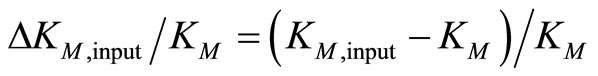 (4)
(4)
 (5)
(5)
The relative deviations of the estimated parameters δKM,est/KM and δkcat,est/kcat are characterized by
 (6)
(6)
 (7)
(7)
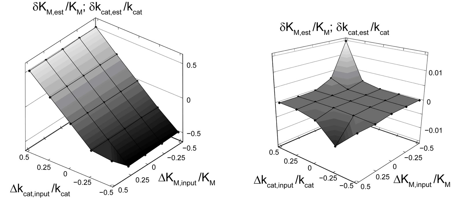
The calculation showed, that the relative deviations of the input parameters in the range of –0.5 ≤ ΔKM,input/KM ≤ 0.5 and −0.5 ≤ Δkcat,input/kcat ≤ 0.5 cause practically equal relative deviations of both estimated parameters:  . Therefore, we combined the results for relative deviations of the estimated parameters KM,est and kcat,est in a single plot, Figure 1.
The results of a direct fit of Equation (3) to the time course P(t) are summarized in Figure 1(a). If the value of kcat,input is somewhat different to the exact value, both KM,est and kcat,est cannot be determined correctly. On the other hand, KM,est and kcat,est are very little sensitive to variations of KM,input. It means that the fit of Equation (3) to P(t) cannot provide convergence to correct values of KM and kcat, if the initial input parameter kcat,input somenwhat deviates from the true value of 650 s–1. As far as we know, all previous attempts to determine KM,est and kcat,est explicitly using Equation (3) were based on the similar approach as tested above [14-16].
We solve this problem by employing the fact that the apparent rate constant in Equation (3) is given by m = kcat·E0/KM [2]. In terms of m, Equation (3) takes the form:
 (8)
(8)
where s = S0 /KM is the dimensionless parameter. Applying Equation (8) to fit kinetics of an enzymatic reaction by nonlinear regression, we render the procedure robust against errors in initial input values of KM and kcat. Using the transformed Equation (8), we obtain very small relative errors for the estimated parameters δKM,est/KM ≈ δkcat,est/kcat in the range between −7.5 × 10⁻³ and 1.5 × 10⁻², Figure 1(b). For the most values of KM,input and kcat,input studied here we calculate even zero deviations. For characterization of the quality of the fit, we use the standard deviation:
 (9)
(9)
where N = 425 is the number of the equidistant time points ti at which the function p(ti) is sampled. Note that when the non-transformed Equation (3) is used, the location of local minima of SD is on a line diagonal to ΔKM,input/KM and Δkcat,input /kcat axis, see Figure 2(a). This is very unfavorable for nonlinear regression and leads to the weak convergence and mainly to a wrong local minimum. The large deviation from the global minimum causes large uncertainty in KM,est and kcat,est. The transformed Equation (8) applied in the new (m, s)-coordinate system exhibits much faster convergence, as Equation (3) in the (KM, kcat)-coordinates, Figure 2(b). Contrary to Equation (3), the fit of the apparent rate constant m at a constant parameter s yields the correct m-coordinate of the global minimum of SD. Fitting s at a correct m-coordinate of the minimum greatly facilitates convergence to the well-defined global minimum of SD shown by the arrow in Figure 2(b). The estimated coordinates mest, sest of the global minimum can be easily recalculated into the parameters KM,est and kcat,est.
 (a) (b)
Figure 1. Hyperplane of the relative deviations of the estimated parameters KM,est and kcat,est from the actual values as a function of the relative deviations of the input parameters ΔKM,input/KM and Δkcat,input/kcat. Black spheres represent calculated points connected by eye-help lines and surfaces. (a) KM,est and kcat,est are estimated using Equation (3). (b) KM,est and kcat,est are estimated using the transformed Equation (8) in the form P(t) = p(t)·S0. Note the large difference in the scales of the vertical axes of (a) and (b). For both plots KM,est and kcat,est are determined by nonlinear regression applied to the error-free function P(t) computed by Equation (3).
 (a) (b)
Figure 2. Standard deviation SD, computed with Equation (9), as a function of the relative deviation of input parameters: DKM,input/KM and Dkcat,input/kcat, (a), and Δsinput/s = (sinput – s)/s, Δminput/m = (minput – m)/m, (b). Black spheres represent calculated values of SD connected by eye-help lines and surfaces. The arrows show the position of the global minima of SD: (a) regression with Equation (3), (b) regression with Equation (8). The error-free functions P(t) and p(t) = P(t)/S0 are computed as specified in Figure 1.
3.2. Advanced Algorithm for Single Trace Regression
The impact of the precision of the input parameters KM,input and kcat,input on the errors on the estimated values of KM,est and kcat,est becomes stronger with increasing noise level of data. Previously, KM,input and kcat,input were determined through a linearization of Equation (3) resulting in uncertain estimates [15,16]. Here we avoid the linearization by using the fact that the simple exponential function
 (10)
(10)
is an approximation to Equation (8), [2]. First, we estimate the input value of the apparent rate constant  via fitting Equation (10) by regression to experimental or simulated p(t) curves. Calculations with simulated p(t) have shown (data are not presented) that for a reliable estimation of
  it is recommendable to sample p(t) up to the maximum time
 . The second input parameter for the dimensionless parameter
  is obtained using the first derivative of Equation (8) for t → 0:
 (11)
(11)
The value (dp(t)/dt)|t→0 ≈ v0,exp is estimated by usual linear regression applied to ten or twenty initial points of the p(t) curve. Rearrangement of Equation (11) gives the second input parameter sinput in the form:
 (12)
(12)
It is recalled that linear regression for v0,exp and nonlinear regression of the exponential Equation (10) for minput yield intrinsically wrong estimates of minput and sinput. However, the estimates are good enough to serve as input parameters for the nonlinear regression with the transformed Equation (8); cf. next Section 3.3. On this way, the determination of minput and sinput can be easily automated; see the reference in the Appendix 1.6. Finally, the searched kinetic constants are given by KM,est = S0/sest and kcat,est = mest·KM,est/E0.
3.3. Robustness of Single Trace Regression to Noise
For testing of robustness of single trace regression to error-prone data, noise was added to the error-free function p(t), Equation (8), in form of the pseudo random error:
 (13)
(13)
where e is the noise amplitude ranging from zero to 0.04, and x is the pseudo-random variable varying in the range of −1 to 1. The function perr (t) is calculated in N = 425 equidistant points in the time range of 0 to 65 s. The estimates mest and sest are determined as averages of five samples of noise of perr (t). As a measure for the quality of the estimations we use the standard deviation, Equation (9). The resulting SD values are small for all noise levels: SD = 0 at e = 0, SD = 5.8 × 10⁻³ at e = 0.01 and SD = 0.024 at e = 0.04. Symmetric distribution of the relative deviations of the estimated parameters δKM,est /KM and δkcat,est/kcat around zero suggests no systematic error in the resulting KM,est and kcat,est values; see Figure 3, right panels.
As mentioned above, the values of δKM,est/KM and δkcat,est/kcat are practically equal to each other in the whole range of ΔKM,input/KM and Δkcat,input/kcat studied here; therefore, they are presented together in the same graph, Figure 3 (right panels). The estimates of KM,est and kcat,est, averaged over the results for 25 input pairs of KM,input and kcat,input, are summarized in Table 1. Note that the estimates are very close to the actual values KM = 220 μM and kcat = 650 s−1, even at e = 0.04.
3.4. Conditions for the Best Convergence
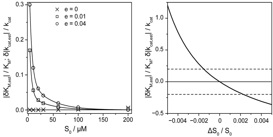
Besides of the noise level of P(t), the quality of analysis depends on the absolute value of the initial substrate concentration S0. To demonstrate the correlation between noise-level and initial substrate concentration, the relative deviation of estimated KM and kcat values as a function of S0 is depicted in Figure 4(a) for three different levels of noise.
The absolute values of the relative deviations of the estimated parameters KM and kcat became larger with decreasing S0 and increasing noise amplitude e. The dependence of |δKM,est|/KM and |δkcat,est|/kcat on S0 can be referred to large rounding errors of the nonlinear regression at small values of initial substrate concentrations, especially when S0 << KM (here at about S0 = 10 µM), and at larger level of noise. Since the parameter s in Equation (8) interrelates S0 to KM, we estimated for a given parameter s the ranges of the apparent rate constant m, which condition a correct determination of KM and kcat. Reliable results of the fit we obtain for s = 0.01 and m between 0.02 and 1.2 s−1, for s = 0.1 and m between 0.024 and 1.9 s−1 as well as for s = 1.0 and m between 0.07 and 1.2 s−1. In that range of the parameters the

Figure 3. Left panels: Progress curves simulated with Equation (8) with parameters as indicated in Figure 1, now with random noise of the amplitudes (a) e = 0, (b) e = 0.01 and (c) e = 0.04. The red lines represent fits with Equation (8) for the calculation of the parameters KM,est and kcat,est. Right panels: Black spheres connected by eye-help lines and surfaces represent the relative deviation δKM,est/KM and δkcat,est/ kcat of the estimated parameters from the actual values as function of the relative deviations of the input parameters ΔKM,input/KM and Δkcat,input/kcat.

Table 1. Estimates of KM and kcat averaged over 25 input pairs KM,input and kcat,input at three different noise levels e. KM and kcat are computed by single trace regression with Equation (8).
 (a) (b)
Figure 4. (a) Absolute values of relative deviations of the estimated parameters KM,est and kcat,est from the actual values as functions of the initial substrate concentration S0 at the three different levels of noise: ×, e = 0.0, □, e = 0.01, and ◊, e = 0.04. The nonlinear regression method was applied to perr(t), see Equation (13), at the input parameters KM,input = 275 μM, kcat,input = 487.5 s−1, corresponding to ΔKM,input/KM = 0.25 and Δkcat,input/kcat = −0.25. (b) The impact of the relative error ∆S0/S0 in initial substrate concentration S0 on the relative deviations |δKM,est|/KM and δ|kcat,est|/kcat of the estimated parameters from the actual values. The solid line represents results of nonlinear regression for the errorfree function p(t); other parameters as in (a). Broken horizontal lines indicate a 20% relative error in KM and kcat.
computation algorithm for Lambert-W function and nonlinear regression implemented in Mathcad 2001 Professional yield exact values of KM,est and kcat,est (data are not shown). The precision of the value of S0 appears to be very important for a correct analysis of progress curves, because of the direct dependence of s on S0. Already the relative deviation ΔS0/S0 = (S0,meas − S0)/S0 of the measured value S0,meas from the exact value S0 in the range ± 0.5% causes a hundredfold larger relative error in the estimated values of KM,est and kcat,est, Figure 4(b). In order to keep the relative error in KM,est and kcat,est within ± 20% error margin, the relative deviation ΔS0/S0 should be in the range between −0.18 and +0.21%. Therefore, the single trace regression requires very precise values of the starting substrate concentrations. Generally, the demanded precision of S0 should be better than about ±0.1%, which is nowadays available in most laboratories.
3.5. Testing v0-Plots and Single Trace Regression with Simulated Data
We tested the limits and quality of the new single trace regression as well as commonly used v0-plots using computer generated data with pseudo-random noise. One source of errors in v0-plots is an inaccurate experimental determination of v0. In our simulations, we determine the realistic error in v0 using a computer simulated trace p(t) with a known level of pseudo-random noise, as opposed to previous computer tests, in which a fixed error was added to v0 [5]. Three classical v0-plots (LineweaverBurk, Eadie-Hofstee and nonlinear) as well as the single trace regression method were applied to the same data set. The results are presented in Table 2 (see also Tables 4 and 5 in Appendix).
Table 2 clearly shows that the single trace regression with Equation (8) yields the most precise results for KM and kcat when error prone simulated data are analyzed.
The nonlinear v0-plot yields good estimates coinciding with actual values within their standard deviations. The Eadie-Hofstee plot yields less accurate results, the estimate does not compare to the true value kcat, even if within the error margin. The Lineweaver-Burk plot yields unrealistic negative values of KM and kcat. Presumably, an uneven distribution of error over S0-values leads to the unrealistic results. This could be to a certain degree corrected by disregarding data points for smaller S0-values, a strategy which is frequently employed by experimentalists exploiting the Lineweaver-Burk plot. Our analysis adheres strictly to all values of the plots to ensure the full comparability of all the methods. We also did not perform a weighting of the data points corresponding to their precision, which additionally may have led to improved results. Another reason for the failure of the Lineweaver-Burk plot is the narrow width of the analyzed S0 range between 3 and 100 μM, compared to the KM-value of 220 μM. Generally, a wider range of S0- values used for analysis increases precision of results of all v0-plots considerably [5]. Regarding this fact, our new single trace regression method could be of great benefit, especially in cases, where a wide range of S0 values cannot be addressed experimentally. As expected, results for a wider range of staring concentrations S0 are more precise, than those for the narrow range of S0-values (see Figure 7 and Table 4 of Appendix). The reason for the notably more precise results of the single trace regression compared to the three v0-plots in Table 2 could be the fact that the initial rates v0 are usually underestimated in their experimental determination (cf. Appendix Figure 6). The effect of the underestimation of v0 on the results of the v0-plots is actually hardly predictable. Dependent on the actual noise level, the estimated values of KM and kcat can be systematically shifted either to lower or to higher values. In that case, the small error margins of KM and kcat are misleading, as demonstrated for the kcat value determined by the Eadie-Hofstee plot in Table 2. Differently to the v0-plots, the results of the new single trace method do not show any systematic deviation from the actual KM and kcat values at all three levels of noise studied here, see Figure 3. In principle, the assessment of KM and kcat can be improved by repeating the single trace experiments and averaging, as opposed to the v0-plots using systematically underestimated values of v0,exp. Therefore, we may conclude that the new method has a potential to yield more precise results than the conventional v0-plots.

Table 2. Comparison of different methods to determine kinetic constants from simulateda enzymatic reactions with noise.
3.6. Testing Single Trace Regression with Experimental Data
To gauge the conventional methods to the single trace regression analysis under experimental conditions of enzymatic catalysis we have chosen the reaction of CcO with ferrous cytochrome c, because at high salt conditions and surplus of oxygen it meets the single substrate Michaelis-Menten model and guarantees full irreversibility of the enzymatic reaction due to formation of water from oxygen during the catalysis as well as the exclusion of product inhibition [18]. The high ionic strengths conditions lead further to slower kinetics of this enzymatic reaction compared to the optimum rate at low ionic strength; see, e.g., review by Cooper [18].
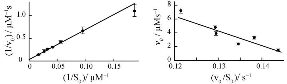
Initial reaction rates v0,exp are measured spectrophotometrically at different starting concentrations S0 of the substrate, ferrous cytochrome c. The corresponding Lineweaver-Burk, Eadie-Hofstee and nonlinear v0-plots are presented in Figures 5(a)-(c).
The resulting kinetic parameters KM and kcat of the plots are summarized in Table 3.
 (a) (b)
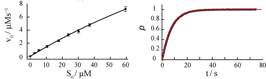 (c) (d)
Figure 5. Four different plots of the kinetic analysis of the reaction of cytochrome c oxidase (E0) with ferrous cytochrome c (S0). Experiments are performed at constant E0 = 50 nM in a 50 mM phosphate buffer, pH = 6.5 and 100 mM KCl. Lineweaver-Burk (a), Eadie-Hofstee (b) plots and nonlinear v0-regression (c) for various cytochrome c initial concentrations S0. Normalized kinetics of the product formation at S0 = 30.08 µM (d). Black circles represent experimental data, the red curve represents Equation (8) with KM = 218 µM and kcat = 645 s−1.
A quantitative comparison of the simulated product curves p(t) at different levels of noise with the experimental p(t) by Equation (9) shows that the experimental level of noise (compared to Table 1) allows for a definite determination of KM and kcat by all three v0-plots studied here. A representative result of a fit of Equation (8) to a single trace of an enzymatic reaction is shown in Figure 5(d). The sevenfold repetition of the single trace regression at seven different S0 values (see Appendix, Table 5) enables computation of standard deviations of KM and kcat in Table 3. It is apparent from the Table 3 that the Lineweaver-Burk plot yields the most imprecise results, what is in line with the conclusion of Hofstee [5]. The nonlinear v0-plot provides the smallest standard deviations of kcat compared with single trace regression or Lineweaver-Burk and Eadie-Hofstee plots. Within the relative large error margin of KM and kcat, the results of the single trace regression are at least consistent with the results of the v0-plots. The variations of the kinetic parameters KM and kcat determined by single trace regression at different substrate concentrations S0 reflect the limits of the method caused by experimental errors; see Table 5 in Appendix. However, the experimental result itself does not suggest any systematic deviations of KM and kcat with S0.
In our experiment it is not clearly evident whether the single trace regression or the v0-plots are generally more precise in determination of kcat and KM. At least we demonstrate here that single trace regression leads to realistic estimates, which are in good agreement with the values of the v0-plots.
4. Conclusions
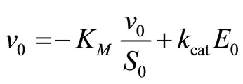
The analytical integration of the Michaelis-Menten Equation (2) in terms of the transformed Lambert-W function, Equation (8), provides a reliable tool to determine the Michaelis-Menten KM and turnover kcat constants from the analysis of a single reaction trace. Supported by our advanced nonlinear regression algorithm, this new method allows determining KM and kcat much quicker than by conventional linearization or by nonlinear plots using a set of (v0,exp, S0) pairs.
The method can be easily implemented as a time and sample saving tool in the online characterization of enzymatic activity. The kinetic parameters KM = 219 ± 4
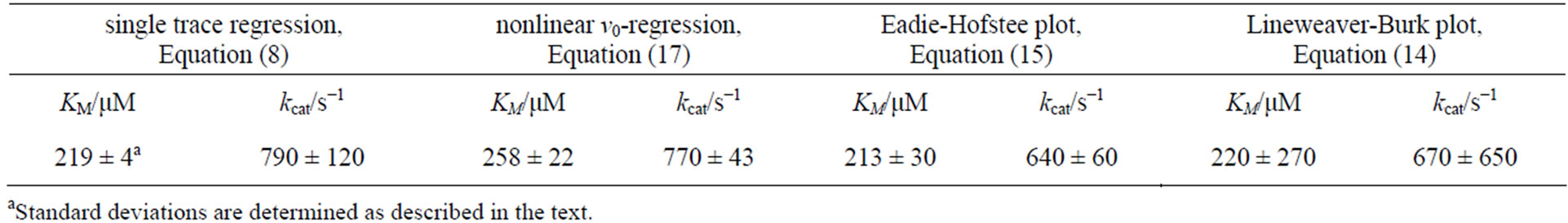
Table 3. Kinetic parameters for the reaction of CcO with ferrous cytochrome c.
μM and kcat = 790 ± 120 s–1 determined with Equation (8) for the CcO reaction are quite conform to results of conventional v0-plots. The fact that no systematic errors occur in KM and kcat in the large range of S0 tested here suggests that application of the single trace method at S0 < KM can complement, if not replace, the conventional methods requiring measurements in the larger range of S0 (0 < S0 < 2 KM, Hofstee (1959), [5]). Note that for some enzymatic reactions, like oxidation of cytochrome c by CcO studied here, the region S0 > 0.5 KM is experimenttally not accessible because the absorption of cytochrome c becomes too strong for correct spectrophotometric determination.
We can therefore expect that the new single trace nonlinear regression will apply to all single substrate irreversible enzymatic reactions whenever a reliable, precise and fast assessment of the kinetic parameters KM and kcat is demanded. The single trace regression with the transformed Lambert-W function can be adopted to analyze reversible enzymatic reactions [21,22], as well as to enzyme kinetics of multiple alternative substrates [23]. In any case, the method will provide a new tool for biotechnology that saves sample and time by reducing the number of experiments at various S0 mandatory for the determination of KM and kcat by v0-plots.
REFERENCES
- L. Michaelis and M. L. Menten, “Die Kinetik der Invertinwirkung,” Biochemische Zeitschrift, Vol. 49, 1913, pp. 333-369.
- S. Schnell and P. K. Maini, “A Century of Enzyme Kinetics: Reliability of the KM and Vmax Estimates,” Comments on Theoretical Biology, Vol. 8, No. 2, 2003, pp. 169-187. doi:10.1080/08948550302453
- G. L. Atkins and I. A. Nimmo, “A Comparison of 7 Methods for Fitting the Michaelis-Menten Equation,” Biochemical Journal, Vol. 149, No. 3, 1975, pp. 775-777.
- R. Walsh, E. Martin and S. Darvesh, “A Versatile Equation to Describe Reversible Enzyme Inhibition and Activation Kinetics: Modeling β-Galactosidase and Butyrylcholinesterase,” Biochimica et Biophysica Acta, Vol. 1770, No. 5, 2007, pp. 733-746. doi:10.1016/j.bbagen.2007.01.001
- B. H. J. Hofstee, “Non-Inverted versus Inverted Plots in Enzyme Kinetics,” Nature, Vol. 184, 1959, pp. 1296-1298. doi:10.1038/1841296b0
- G. E. Briggs and J. B. Haldane, “A Note on the Kinetics of Enzyme Action,” Biochemical Journal, Vol. 19, No. 2, 1925, pp. 338-339.
- H. Lineweaver and D. Burk, “The Determination of Enzyme Dissociation Constants,” Journal of the American Chemical Society, Vol. 56, No. 3, 1934, pp. 658-666. doi:10.1021/ja01318a036
- G. S. Eadie, “The Inhibition of Cholinesterase by Physostigmine and Prostigmine,” Journal of Biological Chemistry, Vol. 146, No. 1, 1942, pp. 85-93.
- G. L. Atkins and I. A. Nimmo, “The Reliability of Michaelis Constants and Maximum Velocities Estimated by Using the Integrated Michaelis-Menten Equation,” Biochemical Journal, Vol. 135, No. 4, 1973, pp. 779-784.
- H. N. Fernley, “Statistical Estimations in Enzyme Kinetics. The Integrated Michaelis Equation,” European Journal of Biochemistry, Vol. 43, No. 2, 1974, pp. 377-378. doi:10.1111/j.1432-1033.1974.tb03423.x
- R. G. Duggleby and J. F. Morrison, “The Analysis of Progress Curves for Enzyme-Catalyzed Reactions by NonLinear Regression,” Biochimica et Biophysica Acta, Vol. 481, No. 2, 1977, pp. 297-312. doi:10.1016/0005-2744(77)90264-9
- F. Liao, X.-Y. Zhu, Y.-M. Wang and Y.-P. Zuo, “The Comparison of the Estimation of Enzyme Kinetic Parameters by Fitting Reaction Curve to the Integrated MichaelisMenten Rate Equations of Different Predictor Variables,” Journal of Biochemical and Biophysical Methods, Vol. 62, No. 1, 2005, pp. 13-24. doi:10.1016/j.jbbm.2004.06.010
- S. Schnell and C. Mendoza, “Closed Form Solution for Time-Dependent Enzyme Kinetics,” Journal of Theoretical Biology, Vol. 187, No. 2, 1997, pp. 207-212. doi:10.1006/jtbi.1997.0425
- C. T. Goudar, J. R. Sonnad and R. G. Duggleby, “Parameter Estimation Using a Direct Solution of the Integrated Michaelis-Menten Equation,” Biochimica et Biophysica Acta, Vol. 1429, No. 2, 1999, pp. 377-383. doi:10.1016/S0167-4838(98)00247-7
- C. T. Goudar, S. K. Harris, M. J. McInerney and J. M. Suflita, “Progress Curve Analysis for Enzyme and Microbial Kinetic Reactions Using Explicit Solutions Based on the Lambert W Function,” Journal of Microbiological Methods, Vol. 59, No. 3, 2004, pp. 317-326. doi:10.1016/j.mimet.2004.06.013
- C. T. Goudar and T. G. Ellis, “Explicit Oxygen Concentration Expression for Estimating Biodegradation Kinetics from Respirometric Experiments,” Biotechnology and Bioengineering, Vol. 75, No. 1, 2001, pp. 74-81. doi:10.1002/bit.1166
- R. Walsh, E. Martin and S. Darvesh, “A Method to Describe Enzyme-Catalyzed Reactions by Combining Steady State and Time Course Enzyme Kinetic Parameters,” Biochimica et Biophysica Acta, Vol. 1800, No. 1, 2010, pp. 1-5. doi:10.1016/j.bbagen.2009.10.007
- C. E. Cooper, “The Steady-State Kinetics of Cytochrome c Oxidation by Cytochrome Oxidase,” Biochimica et Biophysica Acta, Vol. 1017, No. 3, 1990, pp. 187-203. doi:10.1016/0005-2728(90)90184-6
- H.-M. Lee, T. K. Das, D. L. Rousseau, D. Mills, S. Ferguson-Miller and R. B. Gennis, “Mutations in the Putative H-Channel in the Cytochrome c Oxidase from Rhodobacter Sphaeroides Show That This Channel Is not Important for Proton Conduction but Reveal Modulation of the Properties of Heme a,” Biochemistry, Vol. 39, No. 11, 2000, pp. 2989-2996. doi:10.1021/bi9924821
- B. Chance, “Techniques for the Assay of the Respiratory Enzymes,” Methods in Enzymology, Vol. 4, 1957, pp. 273-329. doi:10.1016/0076-6879(57)04060-4
- M. V. Putz, A. M. Lacrama and V. Ostafe, “Full Analytic Progress Curves of Enzymic Reactions in Vitro,” International Journal of Molecular Sciences, Vol. 7, No. 11, 2006, pp. 469-484. doi:10.3390/i7110469
- A. R. Tzafriri and E. R. Edelman, “The Total QuasiSteady-State Approximation Is Valid for Reversible Enzyme Kinetics,” Journal of Theoretical Biology, Vol. 226, No. 3, 2004, pp. 303-313. doi:10.1016/j.jtbi.2003.09.006
- S. Schnell and C. Mendoza, “Enzyme Kinetics of Multiple Alternative Substrates,” Journal of Mathematical Chemistry, Vol. 27, No. 1-2, 2000, pp. 155-170. doi:10.1023/A:1019139423811
Appendix
1. Comparison of the Approaches to Assess KM and kcat
1.1. Linearizations of the Michaelis-Menten Rate Equation
Enzyme kinetics is most commonly analyzed by measuring the initial reaction rate v0 at different substrate concentrations S0. A number of linearization procedures are available for the evaluation of such datasets [3]. Hofstee [5] has pointed out that there is no real basis for the continued use of inverted linearization, like the 1/v0 versus 1/S0, the so-called Lineweaver-Burk plot [7]:
 (14)
(14)
because the plot is sensitive to errors for low and high values of v0 or S0. Eadie [8] and Hofstee [5], proposed to use the v0 versus v0/S0 plot, now commonly known as Eadie-Hofstee plot:
 (15)
(15)
The maximum rate of the product formation is conventionally defined by
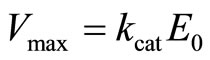 (16)
(16)
1.2. Non-Linearized Michaelis-Menten Equation
Beginning with the wide availability of powerful computers and nonlinear regression software, the Eadie-Hofstee and other linear plots have been partly superseded by nonlinear regression method that should be significantly more accurate and no longer computationally inaccessible. The nonlinear regression method uses the Michaelis-Menten Equation (2) at t→ 0 in the nonlinear form
 (17)
(17)
1.3. Error in the Initial Reaction Rate v0
Practical determination of v0 always leads to underestimated values of the initial reaction rate v0,exp because of the essential non-linearity of the product function P(t) (Figure 6). For instance, if the idealistic curve P(t) is simulated with Equation (3) in N = 425 equidistant points ti from the time region 0 £ t/s £ 65, the sampling time interval is Δt = ti+1 – ti = 0.153 s. If the two first points are used, the “experimental” value v0,exp = (P(t1) − P(t0)) / Δt = 3.866 µM/s is by −0.9% smaller than the correct value v0 = 3.90 µM/s calculated by Equation (17). It is clear, the shorter the interval Δt = t1 − t0, the smaller the difference between v0,exp and v0. Since in experiment the first time point t1 cannot be set arbitrarily close to t0 = 0, the experimental value v0,exp is necessarily smaller than v0. In a more realistic case, when ten initial points are used to calculate v0,exp by linear regression, the underestimation of v0,exp is by −8.2%. It is important to realize, that the initial part of P(t) is an essentially nonlinear function, see insert in Figure 6. Therefore, linear regression does not apply to determine v0. Alternatively, v0,exp can be obtained by fitting a second degree polynomial equation P(t) = at2 + bt + c to the data by nonlinear regression [4]. Extrapolation of the first derivative of the equation to t→ 0 yields v0,exp = b. The nonlinear regression can improve precision of the assessment of v0,exp considerably. Still, the results on v0,exp are very prone to errors in initial estimates of the coefficients a, b and c, as well as to the number of data points and time range taken for the fit. For instance, when ten initial points are used to calculate v0,exp, Figure 6, at the initial parameters a = –0.2 s−2, b = 3 s−1 and c = 0, the underestimation of v0,exp is only −0.14%, at a = −0.5 s−2, b = 1 s−1 and c = 0 the underestimation is −0.16%. When twenty initial points are used to calculate v0,exp, the underestimations are −0.56% and −0.58%, respectively.
1.4. Testing v0-Plots and Single Trace Regression with Simulated Data
For a computational testing of commonly used v0-plots and the single-trace regression we used narrow and wide ranges of starting substrate concentrations S0 (c.f. 2.3 and 2.4). A broader S0-range, up to ~2 KM, is generally favorable for an analysis based on v0-plots compared to the analysis in a narrow range of S0 used for the results presented in Table 2 [5]. In Figure 7 the Eadie-Hofstee (a,d), Lineweaver-Burk (b,e) and nonlinear regression

Figure 6. Product curve (circles) simulated by Equation (3) at KM = 220 µM, kcat = 650 s−1, E0 = 50 nM and S0 = 30 µM for N = 425 equidistant time points with the time interval Δt = 0.153 s. The solid straight line refers to the linear term v0·t, where the initial rate v0 was calculated by Equation (17). The dotted line represents v0,exp·t, where the initial “experimental” rate v0,exp was calculated with the first ten points by linear regression; see inset.

Figure 7. The Eadie-Hofstee (a,d), Lineweaver-Burk (b,e) and nonlinear regression (c,f) plots of the initial rates v0,exp, determined with the first ten points of the simulated relaxation P(t), Equation (3), in the range of S0 from 3 to 100 μM (left column) and of 3 to 500 μM (right column) respectively; see Figure 6 for details. The noise was added to the function P(t) in form of the pseudo-random error of magnitude 2 μM. The solid lines present fits with Equation (14), (a,d), Equation (15), (b,e), and Equation (17), (c,f). The resulting parameters KM and kcat are summarized in Table 3 and in Table 4 of Appendix. The dotted line in (f) indicates the value of the maximum rate Vmax = 32.5 µM/s.
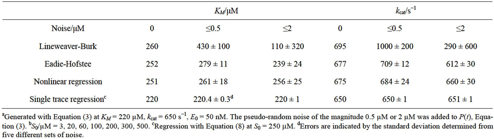
Table 4. Kinetic parameters determined by different methods from simulated dataa with pseudo-random noise for a wide range of S0b.
v0-plots (c,f) are shown for the S0-range from 0 to 100 µM (left side) and from 0 to 500 µM (right side), respectively. Notably, the KM-value for the simulations was set to 220 µM. The diagrams are based on data generated by the simulation of the enzymatic product curve P(t) with Equation (3) and a noise magnitude of 2 µM.
It is evident in Figure 7 that the data points obtained in the broad range of S0 (d,e,f) deviate less from the regression curves compared to the respective plots obtained for the narrower S0-range (a,b,c). This observation is consistent with results of the corresponding plots presented in Table 4. Standard deviations of the KM and kcat values in Table 4 are significantly smaller compared to the corresponding deviations in Table 2. Additionally to Table 2, in Table 4 the results of simulations at the noise-magnitudes of 0 and 2 µM are presented too. However, the general features of the impact of the S0-range on quality of the analysis are throughout the same as in Table 2. The Lineweaver-Burk plot does not yield unphysical, negative results, yet provides the most imprecise results compared to other v0-plots. The Eadie-Hofstee and the nonlinear regression plot yield considerably more precise results than the Lineweaver-Burk plot. However, all v0-plots are not able to correctly determine the true values of KM and kcat in the range of their standard deviations. At low noise-magnitudes, the results of the v0-plots are generally overestimated. With increasing noise-level, this effect may be (over-) compensated by imprecision of results.
As in the case of the narrow S0-range, the single trace regression method yields reasonable results for all investigated noise-magnitudes and shows only nonsystematic errors of the determined KM and kcat values (see Table 4).
1.5. Testing v0-Plots and Single Trace Regression with Experimental Data on CcO
The single trace regression method is able to determine KM and kcat for every single time course of an enzymatic reaction at a single S0-value, contrary to commonly used v0-plots. In our case, the KM and kcat parameters are determined for time traces of the enzymatic reaction of CcO with ferrous cytochrome c at seven different S0- values ranging from 2.68 to 59.35 µM. The results of the new regression method are presented in Table 5; the corresponding mean values and standard deviations of KM and kcat are shown in Table 3. For the experimental curves no systematic deviations of the resulting KM and kcat are observed, as for the simulated data.

Table 5. Results of single trace regressiona of the enzymatic reaction of CcO with cytochrome c at different initial substrate concentrations S0.
1.6. Mathcad Code for Michaelis-Menten-Lambert Analysis of a Single Progress Curve of Enzyme Kinetics
The complete Mathcad code for analysis of single progress curves of enzymatic reactions with the MichaelisMenten-Lambert equation can be found on the homepage of the corresponding author:
http://www.uni-bielefeld.de/chemie/arbeitsbereiche/pc3-hellweg/work/sergej/MathcadCode.pdf The Mathcad code begins with a generation of the Lambert-W function W(x). For this purpose we use the standard Mathcad function “wurzel” to solve the equation yey – x = 0 with an initial value of y = 0.1 and tolerance = 10−15.
a) The second part of the code starts with an input of the total substrate concentration S0 as well as the total enzyme concentration E0, and the upload of an experimental product progress curve P(t).
b) An initial value of the apparent rate constant m is estimated from the experimental normalized product curve p(t) = P(t)/S0. Here we use the exponential approximation  and the 2/3-amplitude criterion to estimate the characteristic relaxation time t = 1/m of p(t). To obtain a more precise estimate of m we use the initial estimate of m further as an input parameter for a nonlinear fit of pexp(t) to the experimental product curve p(t). Therefore, the standard function “Minfehl” implemented in Mathcad is applied.
c) An initial reaction rate v0 of the product curve p(t) is determined by the standard function “neigung” using the first 11 points of p(t).
d) An estimate of the dimensionless input parameter s is calculated by s = |m/v0 − 1|.
e) Exact values of the Michaelis-Menten parameters KM and kcat are determined by the “Minfehl” function using the experimental p(t)-curve and the estimates of m and s as input parameters.
In the third part, the calculated Michaelis-Menten parameters KM, kcat and Vmax are summarized together with results of the fit of the integrated Michaelis-Menten Equation (8) to the experimental p(t)-curve.
Abbreviations
CcO: cytochrome c oxidase;
E0: Total enzyme concentration;
S0: Starting substrate concentration;
kcat: Catalytic constant, a key parameter in enzymatic analysis;
KM: Michaelis-Menten constant, a key parameter in enzymatic analysis;
KM,input, kcat,input: Input parameters for KM and kcat for their estimation by nonlinear regression;
KM,est, kcat,est: Estimated values of KM and kcat by nonlinear regression;
m: The apparent rate constant, defined as m = kcat·E0/KM;
s: The dimensionless parameter, defined as s = S0/KM;
P(t): Progress curve of the product concentration of an enzymatic reaction;
p(t): Normalized product concentration, defined as p(t) = P(t)/S0, ranging from 0 to 1;
v0: Initial reaction rate of the progress curve;
v0-plots: Methods for analyzing enzyme kinetics based on a variety of initial rates v0 at different S0.