Open Journal of Forestry
Vol.09 No.03(2019), Article ID:93177,19 pages
10.4236/ojf.2019.93010
Using Biophysical Variables and Stand Density to Estimate Growth and Yield of Pinus patula in Antioquia, Colombia
Héctor I. Restrepo1*, Sergio A. Orrego2, Juan C. Salazar-Uribe2, Bronson P. Bullock1, Cristian R. Montes1
1Plantation Management Research Cooperative, Warnell School of Forestry and Natural Resources, University of Georgia, Athens, GA, USA
2Universidad Nacional de Colombia, Medellín, Colombia
![]()
Copyright © 2019 by author(s) and Scientific Research Publishing Inc.
This work is licensed under the Creative Commons Attribution International License (CC BY 4.0).
http://creativecommons.org/licenses/by/4.0/


Received: May 6, 2019; Accepted: June 21, 2019; Published: June 24, 2019
ABSTRACT
Timberland investment opportunities in Colombia are expected to increase as a result of the peace agreement recently signed between the Colombian government and the Revolutionary Armed Forces of Colombia. This new socio-political environment may facilitate the expansion of commercial forest plantations on a wider range of site conditions that are currently considered in existing biometric tools. Data from 1119 temporary plots of unthinned, unmanaged, and genetically unimproved Pinus patula plantations in the Antioquia region were combined with a large set of biophysical attributes to identify spatial variation in yield. A wide array of biophysical covariates was explored to characterize the most favorable environmental conditions for the species, and to identify potential explanatory variables to be included in forest yield models. The mathematical form of the model is the von Bertalanffy-Chapman-Richards type, with parameters: asymptote, intrinsic growth rate and allometric constant. The parameters were expressed as linear functions of soil pH, terrain slope, the mean annual temperature to mean annual precipitation ratio, and stand density. The statistical contribution of selected covariates was evaluated using the likelihood ratio test. The model was validated using an independent set of 133 observations. The spatial representation of the model depicts the timber production potential and allows for the identification of the most suitable geographical areas to establish Pinus patula plantations in Antioquia, Colombia. The estimated yield model provides a reliable baseline for timber production, and insight into timberland investments in Colombia.
Keywords:
Von Bertalanffy, Chapman-Richards, Fixed-Effect Models, Forest Productivity, Mexican Pine, Mean Annual Increment

1. Introduction
The end of the 50-year internal armed conflict in Colombia, resulting from the peace agreement signed between the Colombian Government and the Revolutionary Armed Forces of Colombia, is expected to lead to a substantial social-economic transformation. Increased private and public investments are expected to boost the domestic economy. Timberland investments have received considerable attention due to land availability, relatively high rates of forest growth, and the strategic geographical location of Colombia (Cubbage et al., 2010; Cubbage et al., 2007; López et al., 2010; Mendell et al., 2006) . Antioquia is the Colombian state with the largest area in forest plantations with 69000 ha, and a region characterized by a high timber production potential, an increasing demand for timber, and a high economic development. These potential timberland investments require appropriate growth and yield modeling, which provides valuable inputs for performing financial analysis and risk assessment (Hall & Bailey, 2001; Louw, 1999; Moser & Hall, 1969) .
Forest growth is a function of four factors (Clutter et al., 1992) : 1) the stand age, 2) the site quality or environmental effect (Bravo-Oviedo et al., 2007; Louw & Scholes, 2006) ; 3) the intrinsic characteristics of a forest stand, such as density and tree genetics (Calegario et al., 2005) ; and 4) management practices such as mechanical site preparation, fertilization, and competing vegetation control (Allen et al., 2005) . The effect of age on forest growth is accounted by for the inclusion of the stand age in the growth and yield models. Moreover, one of the intrinsic characteristics, density, is accounted by for the planting density, survival/mortality model or stand density.
Much research has been devoted to site quality since it represents a measure of the base timber production potential of a stand. The determination of the site quality is particularly important in Colombia, where intensive forest management practices such as mid-rotation cultural treatments, sustained fertilization and vegetation control, and planting genetically improved seedlings have not been extensively applied. Site quality can be analyzed by either direct or indirect methods.
The direct method to determine forest productivity requires measuring plots in stands representing distinct ages and site qualities, and estimating a site index equation based on dominant heights (Burkhart et al., 2018; Clutter et al., 1992; Walters et al., 1989) . Nevertheless, this approach has some shortcomings: the existence of forest plantations is required to assess site productivity; estimations are locally restricted, and the actual effect of the environment on forest production and productivity is not analyzed. Moreover, the assumption of independence between planting density and dominant height cannot be satisfied (Antón-Fernández et al., 2011; Henskens et al., 2001; Land et al., 2004) , thereby providing biased estimations of forest productivity. Virtually all existing forest growth and yield (FG&Y) models for P. patula in Colombia utilize the site index as their primary input, precluding yield estimations on a regional scale.
On the other hand, the indirect method or geocentric approach (Weiskittel et al., 2011) of forest productivity is intended to estimate growth and yield models as a function of the site quality factors: climate, soil, and topographic conditions (Bravo-Oviedo et al., 2007; Clutter et al., 1992; Günter et al., 2009; Louw & Scholes, 2002, 2006; Lugo et al., 1988; Palahi et al., 2004; Vanclay, 1992; Walters et al., 1989; Wang et al., 2005; Zapata-Cuartas, 2007) .
Models based on an explicit biological explanation of FG&Y are more appropriate than empirical models (Vanclay, 1994) . The von Bertalanffy-Chapman-Richards (vBCR) model has a well-grounded biological basis with its mathematical terms implicitly expressing the underlying physiological processes occurring in an organism. The vBCR model has been extensively examined worldwide for many species (Buford & Burkhart, 1987; Fekedulegn et al., 1999; Moser & Hall, 1969; Pienaar & Turnbull, 1973; Pienaar, 1979; Zeide, 1993) , as well as in Colombia for Acacia mangium (Torres & del Valle, 2007) , Eucalyptus sp. (Zapata-Cuartas, 2007) , Pinus patula (Restrepo et al., 2012) , and Tectona grandis (Restrepo & Orrego, 2015; Restrepo et al., 2012; Torres et al., 2012) . Likewise, the vBCR parameters have been expressed as a function of covariates (Bravo-Oviedo et al., 2007; Hall & Bailey, 2001; Louw & Scholes, 2006) .
P. patula was chosen to characterize the timberland investment potential because this species is the most widely planted in Colombia (Endo, 1994) , as well as in Antioquia where the planted area is 20000 ha (DANE, 2004) . The natural range of P. patula is the south-central region of Mexico (Webb et al., 1984) . However, P. patula has been planted worldwide in a wider climatic range than its natural habitat (van Zonneveld et al., 2009) . Biophysical covariates associated with the three forest growth factors have been utilized to explain P. patula FG&Y variation (Evans, 1974; Grey, 1979; Louw & Scholes, 2006) .
This research had three main objectives. First, to explore a large set of covariates, and to select a subset that potentially explain P. patula growth and yield variation in Antioquia, Colombia. Second, to estimate and validate a P. patula FG&Y model as a function of stand age, stand density, and selected biophysical variables using the vBCR model. Our hypothesis is that the stand age and density, along with biophysical covariates representing site quality factors will explain P. patula growth and yield in Antioquia, Colombia. Third, to spatially represent P. patula FG&Y in Antioquia, Colombia. The resulting map will be useful to provide insight into potential areas for timberland investment in the region.
2. Methods
2.1. Data
The database of forest measurements comprises 1119 1/40 ha-circular-geo-referenced temporary plots measured in unthinned, unmanaged, and genetically unimproved P. patula plantations in eight locations in Antioquia, Colombia (Table 1). Data correspond to forest inventories conducted by the Department of Forest Sciences at National University of Colombia, Medellin, in forest plantations of Empresas Públicas de Medellin, and by students conducting a Forest Engineering thesis in forest plantations of Cipreses de Colombia (Lopera & Gutiérrez, 2000) . Raster maps for climatic variables and a digital elevation model were obtained from WorldClim, version 1.4 (Hijmans et al., 2005) , and the Shuttle Radar Topography Mission (Farr et al., 2007) , respectively. Soil data, including the pH level, were obtained in vector format from national public databases in Colombia (IGAC, 2007) (Table 1). Additional covariates were calculated with the collected dataset. The slope of the terrain (S, degrees) was calculated from the digital elevation model using the d-eight algorithm as implemented in the R function terrain (Hijmans et al., 2016) using a 30 m grid size DEM. The temperature to precipitation ratio (TP, 100˚C∙mm−1) was calculated as:
, (1)
where Amt is the annual mean temperature (˚C), and Amp is the annual mean precipitation (mm), and the value of 100 is a scale factor.
2.2. Model Description
The integrated form of the vBCR model can be written as:
, (2)
where y is the yield volume (m3∙ha−1), f is the asymptote (m3∙ha−1), A is the stand age (years), β is the intrinsic growth rate, and γ is the allometric constant. The parameters f and β represent the potential environmental effects on growth and yield since they are related to metabolic outcomes of resource availability (Brown & Lugo, 1982; González, 1994; Lugo et al., 1988; Pienaar, 1979) . The parameter γ represents, theoretically, a characteristic growth attribute for a species (González, 1994; Pienaar & Turnbull, 1973) and, therefore, it is not related to environmental variables. The parameter γ, generally found in the range [0,2], adds flexibility to the vBCR model (Richards, 1959) . Thus, a value of γ greater than 1 corresponds to a logistic shape for the yield curve; when γ is less than 1, it corresponds to the Mitscherlich curve; when γ is equal to 1, the model takes the name of Gompertz function (Pienaar & Turnbull, 1973; Zapata-Cuartas, 2007) . Additionally, the γ parameter is related to the curve’s inflection point and to the age at which the maximum current annual increment is attained, thereby influencing both the biological and economical rotation ages.
2.3. Model Estimation and Validation
Equation (2) was estimated using generalized nonlinear least-squares with the R function gnls with the variance function argument as varPower (Pinheiro et al., 2017) . Different parameter linear specifications as a function of age, stand

Table 1. Summary statistics of the 1119 temporary plots of P. patula and environmental covariates in Antioquia, Colombia.
density and biophysical covariates were evaluated. The first estimated model expressed the volume as a function of the parameters f, β, γ, and age. Out of this formulation, nested models were specified by expressing each parameter as a function of an intercept, the stand density, and one or more biophysical covariates. The same biophysical covariate was not considered in more than one parameter to avoid potential multicollinearity.
The statistical contribution of one additional covariate in the nested models was evaluated using the likelihood ratio (LR) test (Wackerly et al., 2008) :
(3)
where θ represents the vector of parameters, i.e. f, β, γ; and w and Ω represent the parameter space of the models with p − 1 and p parameters, respectively. The estimated model containing p parameters was compared to the previous model containing p − 1 parameters. For a large number of observations, −2 log(LR) has approximately a distribution. The rejection region is defined as , with for a level of significance .
The validation was performed using an independent 133-observation dataset of forest plantations (ICA, 2015) with similar biophysical attributes and stand characteristics of the measured plots. Specifically, the hypothesis tested was:
where µo is the mean of observed volume and µf is the mean of fitted values, estimated by their corresponding sample means , and , respectively. The test statistics is:
(4)
where and are the sample variances of the observed volumes and fitted values, respectively. Hence, the null hypothesis of equal means is rejected if , with t(0.975, 264) = 1.969 for a level of significance .
2.4. Forest Growth, Yield Curves and Yield Map
Parameters f and β were estimated for each of the 1119 plots based on the covariate values associated with each location. The mean and the 95% prediction interval (2.5% and 97.5% percentiles of the distribution) for these two parameters were estimated to depict the mean and the 95% prediction interval of the growth and yield. The parameter γ was fixed in all these calculations because it does not vary across the study area or as a function of the stand density. Similarly, parameters f and β were represented as a function of the mean of covariates and were used to generate a map of forest yield at year 20. Natural protected areas, which include lands above 2800 meters above sea level (m.a.s.l.), were not considered in the analyses and maps (Gómez-Ossa, 2011) , given the environmental restrictions by which forest plantations are not allowed as land use on protected areas.
3. Results
3.1. Biophysical Covariates Description and Variable Selection
The measured plots in Antioquia represent climatic conditions of Amt, Amp, and TP at (mean ± SD) 17.5˚C ± 1.0˚C, 2508 ± 681.2 mm, 0.74 ± 0.18 100˚C∙mm−1, respectively. Soil and topography were characterized by the mean terrain slope at 14.7 ± 6.6 degrees, and soil pH mainly between 5.1 and 6. Most biophysical covariates exhibited a bell-shape relationship with parameters f and β, providing empirical evidence of optimal environmental conditions for P. patula in Antioquia. For instance, parameters f and β exhibited their maximum values for Amt and Amp at 17.5˚C and 2200 - 2500 mm∙yr−1, respectively (Figure 1 and Figure 2). Similar bell-shape curves, showing the maximum values for f and β, were exhibited for other biophysical covariates, e.g. moister quarter’s precipitation (Mqp), coolest month’s temperature (Cmt), and moister month’s precipitation (Mmp) (Figure 1 and Figure 2).
Points in Figure 1 and Figure 2 are assumed to represent the average contribution of a covariate to the parameters f and β within one of the eight locations. Similarly, the lines show the general trend (a loess smoother) of the relationship of the covariable and parameters f and β (§8.2.2 Using covariates with nlme in Pinheiro & Bates, (2000) ). Thus, a line with a noteworthy trend and relative high gradient (how steep the line is) makes the covariate a good candidate to be selected as potential explanatory variable. Both the soil pH (difference between pH levels) and terrain’s slope (steeper than 15˚) contribute with more than 100 m3∙ha−1 to the asymptote (f) (Figure 1). TP has a noticeable trend with high gradient, suggesting that the higher the TP the higher the intrinsic growth rate (b) (Figure 2).
Overall, pH, S, and TP capture the effect of both f and β, and for that reason they were chosen over the remaining covariates. These variables were plotted in the first row of Figure 1 and Figure 2, along with stand density (N), to help the reader to identify described relationships with the parameters. Moreover, the selected biophysical covariates can be easily determined by practitioners and researchers from field measurements or publicly available data without much need of additional external inputs or further complex calculations.
3.2. Yield Model
In the best estimated model, the parameter f was a function of an intercept, pH, S, and N; the parameter β was a function of an intercept, and TP; and the parameter γ was a function of just an intercept (Table 2, model 20). This model had the maximum value of the log likelihood (Table 2), and its parameter estimates were highly statistical significant (p-value < 0.001) (Table 3). The parameter estimates can be written as (Table 3):
, (5)
(6)
(7)
where represents an indicator function that takes the value of one if the soil pH is in the range 5.1 - 6, or zero otherwise (in this case the remaining option is soil pH between 4.1 and 5).
The asymptote f is expressed as a function of an intercept, equal to 236 m3∙ha−1, and the effect of two covariates, pH and S. On sites where pH was in the range 5.1 - 6, the asymptote was lower in 112.4 m3∙ha−1 compared to sites where pH was in the range 4.1 - 5. Moreover, each additional degree of slope added 2.2
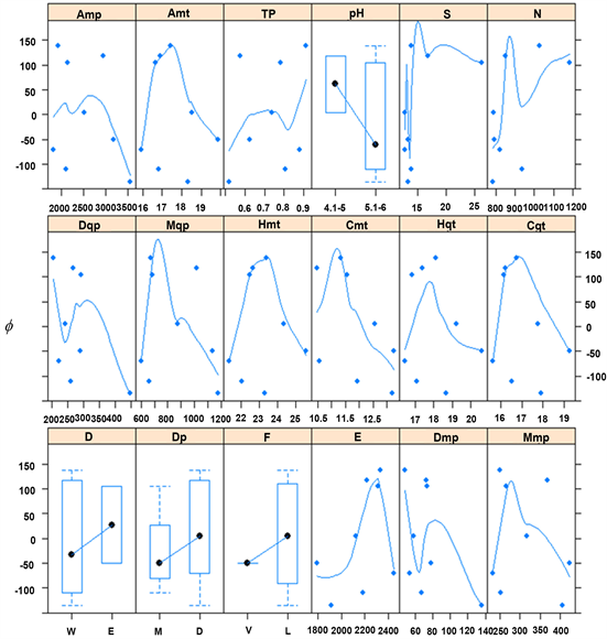
Figure 1. Relationship between the parameter f with environmental covariates and stand density: Amp, annual mean precipitation (mm∙yr−1); Amt, annual mean temperature (˚C); TP, temperature to precipitation ratio (100˚C∙mm−1); pH, soil pH class; S, slope of the terrain (degrees); N, stand density (trees per ha); Dqp, driest quarter’s precipitation (mm∙Qtr−1); Mqp, moister quarter’s precipitation (mm∙Qtr−1); Hmt, hottest month’s temperature (˚C); Cmt, coolest month’s temperature (˚C); Hqt, hottest quarter’s temperature (˚C); Cqt, coolest quarter’s temperature (˚C); D, soil drainage class (W: well; E: excessive); Dp, soil depth class (M: moderate, <80 cm, D: deep, >80 cm); F, soil fertility class (V: very low; L: low); E, elevation (meters above sea level, m.a.s.l.); Dmp, driest month’s precipitation (mm∙mo−1); and Mmp, moister month’s precipitation (mm∙mo−1).
m3∙ha-1 to the asymptote. Regarding density, for each 100 standing TPH, the asymptote increases in 18 m3∙ha−1. The parameter β was expressed as a function of an intercept, equal to −0.123, and TP. As described, the higher the TP, the higher the value of . Evidence was not found to reject the null hypothesis that the mean of observed and estimated volumes of the validation dataset were different (p-value > 0.05).
The average growth and yield curves of P. patula by soil pH are shown in b. Figure 3(a) depicts the average yield with parameter estimates of = 432.578 and = 0.266; and = 312.624 and = 0.292 for locations where soil pH is in the range 4.1 - 5 and 5.1 - 6, respectively. The parameter estimate was constant for both soil pH factor levels. The estimated yield curves are flat over
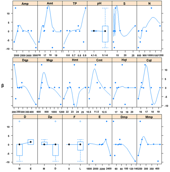
Figure 2. Relationship between the parameter β with environmental covariates and stand density: Amp, annual mean precipitation (mm∙yr−1); Amt, annual mean temperature (˚C); TP, temperature to precipitation ratio (100˚C∙mm−1); pH, soil pH class; S, slope of the terrain (degrees); N, stand density (trees per ha); Dqp, driest quarter’s precipitation (mm∙Qtr−1); Mqp, moister quarter’s precipitation (mm∙Qtr−1); Hmt, hottest month’s temperature (˚C); Cmt, coolest month’s temperature (˚C); Hqt, hottest quarter’s temperature (˚C); Cqt, coolest quarter’s temperature (˚C); D, soil drainage class (W: well; E: excessive); Dp, soil depth class (M: moderate, <80 cm, D: deep, >80 cm); F, soil fertility class (V: very low; L: low); E, elevation (meters above sea level, m.a.s.l.); Dmp, driest month’s precipitation (mm∙mo−1); and Mmp, moister month’s precipitation (mm∙mo−1). Values of the vertical axis in 100.000 units.
the first four years, increasing steadily until year 25. The average mean annual increment (MAI) reaches a maximum of 22.7 and 18.0 m3∙ha−1∙year−1 at years 15 and 13 for pH 4.1 - 5 and 5.1 - 6, respectively (Figure 3(b)). The shading region in each panel of Figure 3 represents the 95% prediction interval (PI) by the two pH factor levels, describing the growth and yield variability associated with the environmental covariates considered. For example, the MAI’s 95% PI was (11.21, 43.27), and (5.28, 38.84) m3∙ha−1∙year−1 for soil pH 4.1 - 5, and 5.1 - 6, respectively. Overall, the 95% PI of biological rotation age was in the range of 9 - 30 years (Figure 3(b)).
The spatial representation of the parameters f and β, and the yield is presented in Figure 4. The map of the parameter f indicates that the most productive areas
Table 2. Estimated yield models of P. patula in Antioquia, Colombia.
int: intercept; LR: likelihood ratio; soil pH (pH, dummy variable with value of one for pH in the range 5.1 - 6, and value of zero for pH in the range 4.1 - 5), slope (S, degrees), temperature to precipitation ratio (TP, 100˚C∙mm−1), and stand density (N, trees per hectare (TPH)).
Table 3. Parameter estimates for the yield model of P. patula.
int: intercept; soil pH (pH, dummy variable with value of one for pH in the range 5.1 - 6, and value of zero for pH in the range 4.1 - 5), slope (S, degrees), temperature to precipitation ratio (TP, 100˚C∙mm−1), and stand density (N, trees per hectare(TPH)).

Figure 3. Growth and yield of Pinus patula in Antioquia, Colombia. (a) volume yield (m3∙ha−1) as a function of age by soil pH; (b) mean annual increment (m3∙ha−1∙yr−1) as a function of age soil pH. The solid and dashed lines correspond to the average curve for pH 4.1 - 5 and 5.1 - 6, respectively, and the shading region represents their 95% prediction intervals.
are located in the northeastern region of Antioquia (Figure 4(a)). High values of the parameter β are observed in the central region of Antioquia (Figure 4(b)). At age 20 years, the spatial representation suggests that the yield is high in some areas of the northeastern region of Antioquia (Figure 4(c)). The total suitable land for planting P. patula in Antioquia is 10,600 km2.
4. Discussion
Biophysical conditions that contribute with the optimal growth of P. patula in Antioquia are similar to those found in the natural range of the species: annual mean temperature in the range of 12˚C - 18˚C, mean maximum temperature of the hottest month in the range of 20˚C - 29˚C, mean minimum temperature of the coldest month in the range of 6˚C - 12˚C, and annual mean precipitation in the range of 750 - 2000 mm∙year−1 (Gillespie, 1992; Webb et al., 1984) . We explored the effect of a wide array of biophysical covariates on P. patula growth and yield. Forest yield models expressing stand volume of P. patula as a function of environmental covariates were not found in previous studies. Virtually all existing FG&Y models that include the effect of biophysical covariates utilize dominant height or site index as dependent variables. Site index has been expressed as a function of the relative distance between the summit and the plantation site, elevation, slope, soil quality (Evans, 1974) , parent material, soil pH, effective soil depth (Grey, 1979) , nitrogen mineralization, topographic position and soil classification (Louw & Scholes, 2006) . Moreover, the main variables of a climate envelope model for P. patula were, in order, annual mean temperature,

Figure 4. Spatial representation of the estimated parameters of the yield model of P. patula in the altitudinal range of 1800 - 2800 m.a.s.l. and after excluding protected areas: (a) Asymptote (m3∙ha−1) or parameter f in the estimated model; (b) Intrinsic growth rate or parameter β in the estimated model; (c) Estimated yield (m3∙ha−1) at year 20.
the maximum temperature in the warmest month, annual precipitation, precipitation in the driest month, temperature seasonality, and annual temperature range (Leibing et al., 2013; van Zonneveld et al., 2009) . The driest quarter’s precipitation has been found as a relevant variable to explain P. patula growth as well (Louw & Scholes, 2006) .
Data used to estimate the FG&Y model corresponded to unthinned, unmanaged and genetically unimproved forest plantations, and characterized P. patula plantations in Antioquia and other regions of Colombia as well. The vBCR model can be estimated using data from temporary plots representing contrasting environmental conditions (Pienaar & Turnbull, 1973) , like the data used in this research. The asymptote (f) and intrinsic growth rate (β) parameters in the vBCR have a well-known relationship with environmental covariates (Louw, 1999; Louw & Scholes, 2002, 2006) .
Out of the biophysical covariates explored, we selected soil pH, terrain slope, the temperature to precipitation ratio because they exhibited a distinct relationship with parameters f and β. We considered TP as a reasonable explanatory variable for P. patula growth, as studies on tropical forest growth suggest that total biomass is explained by TP (Brown & Lugo, 1982) . This index reflects the water availability to plants due to potential evapotranspiration that is proportional to air temperature (Lugo et al., 1988) . Likewise, since TP can easily be calculated using Amt and Amp, it represents a good index to be used by practitioners and investors compared to other measures like the water deficit index. Regarding soil pH and slope as soil and topographic factors, respectively, they are found to influence forest production and their corresponding asymptote in yield models (Evans, 1974; Grey, 1979; Louw & Scholes, 2006) . These biophysical covariates can be easily obtained from field measurements, facilitating the forest productivity evaluation. The finding that no covariate was related to the parameter γ is supported by the theory that the allometric constant is directly related to the way in which a specific species can grow and survive (Pienaar & Turnbull, 1973) .
Density is usually assumed to be more related to the intrinsic growth rate than to the asymptote (Pienaar & Turnbull, 1973) . However, stand density was found to be an explanatory variable related to the asymptote. In this case, the relationship between stand density and the asymptote may be the result of the effect of contrasting environmental conditions on the stand survival rates.
The estimated asymptotes in this study are in the range of maximum volume values previously reported for P. patula in Latin America: 360 m3∙ha−1 at year 48 in Colombia (Ramírez et al., 2014) , and 180 - 350 m3∙ha−1 at year 40 in Mexico (Santiago-García et al., 2014) ; but less than the maximum volume values reported in Africa: 550 m3∙ha−1 at year 31 in Ethiopia (Lemenih et al., 2004) ; and 900 ± 50 m3∙ha−1 at year 41 in Angola (Delgado-Matas & Pukkala, 2012) . However, these maximum values of volume correspond to average potential timber production and seem to be related to one location or one small area. That is the case of a volume value of 843 m3∙ha−1 at year 25 contained in our dataset (Table 1).
The 95% prediction intervals of the forest yield and MAI suggest a high variability in timber production for P. patula plantations in Antioquia, Colombia. The range of the maximum MAI and its associated biological rotation are wider than previously reported (Table 4). The observed variability of the growth and yield of P. patula leads to considerable uncertainty, thereby having significant implications for financial profitability and risk of timberland investments (Restrepo et al., 2012) .
The estimated model can be considered as a baseline for analyzing timber production in Antioquia, Colombia, by using data from unthinned, unmanaged, and genetically unimproved P. patula plantations. Hence, the potential timber
Table 4. Mean annual increment and biological optimal rotation for P. patula.
aMaximum MAI and biological rotation, b95% prediction interval; cIt is a conversion of mean annual biomass increment of 14 ton∙ha−1∙yr−1 to mean annual increment using a value of density of 400 kg∙m−3.
production is likely to be higher under intensive forest management practices. The estimated model can be used to estimate and predict the yield of P. patula in other Colombian regions with environmental conditions similar to those represented in this research. However, it is strongly recommended to use forest inventory data and independent forest yield models to validate those estimations.
5. Conclusion
A broad range of environmental conditions was used to estimate the vBCR model type for FG&Y. The modeling approach explicitly includes biophysical covariates, and contributes to the identification of the main drivers of P. patula growth in Antioquia, Colombia. The asymptote (f) was estimated as a function of soil pH, slope of the terrain and stand density. The intrinsic growth rate (β) was estimated as a function of the temperature to precipitation ratio. The latter is a very interesting and promising, ecological-theoretical index to be used in FG&Y studies regardless of the species. Moreover, since the model includes climate variables, it can be used to examine potential effects of future climatic conditions on FG&Y. Although more biophysical covariates representing site quality factors were examined, they were not included in the model because they may explain the same variability as selected covariates. Moreover, selected biophysical covariates can be obtained easily from field measurements taken by practitioners, when they conduct technical feasibility studies of timberland investments. The allometric constant (γ) was not related to environmental covariates because it reflects the species’ autoecology of growth. Lower and upper bounds of the 95% prediction intervals for growth and yield were determined as a function of the parameters f and β. The results suggest that FG&Y of P. patula is highly variable, which has significant implications for financial profitability and risk evaluation in forest plantations. The estimated parameters f and β, and yield of P. patula were represented in maps to identify the most suitable areas where P. patula can be planted in Antioquia. The estimated model, growth and yield curves, and forest yield maps provide valuable information for timber investment analysis. Future research should address other important drivers of FG&Y such as genetics and silvicultural treatments to determine volume gains associated with intensive forest management practices.
Acknowledgements
This research was funded by the Project “Determinantes Espacialmente Explícitos de Transiciones en Coberturas Terrestres con Significativo Impacto para la Provisión de Servicios Ecosistémicos”, which is part of the research program “Gestión del Riesgo por Cambio Ambiental en Cuencas Hidrográficas”, funded by Colciencias. We sincerely thank to Cesar Urrego, Álvaro Lema, Rodolfo Parra, Victor Gutiérrez, Gabriel Lopera, Ingrid Mazo, Juan David Arango, and Astrid Gil for their invaluable contribution to this research. We also would like to thank the foresters, technicians and people who were directly responsible for field measurements which were used to consolidate the dataset for this research.
Conflicts of Interest
The authors declare no conflicts of interest regarding the publication of this paper.
Cite this paper
Restrepo, H. I., Orrego, S. A., Salazar-Uribe, J. C., Bullock, B. P., & Montes, C. R. (2019). Using Biophysical Variables and Stand Density to Estimate Growth and Yield of Pinus patula in Antioquia, Colombia. Open Journal of Forestry, 9, 195-213. https://doi.org/10.4236/ojf.2019.93010
References
- 1. Allen, H. L., Fox, T. R., & Campbell, R. G. (2005). What Is Ahead for Intensive Pine Plantation Silviculture in the South? Southern Journal of Applied Forestry, 29, 62-69. [Paper reference 1]
- 2. Antón-Fernández, C., Burkhart, H. E., Strub, M., & Amateis, R. L. (2011). Effects of Initial Spacing on Height Development of Loblolly Pine. Forest Science, 57, 201-211. [Paper reference 1]
- 3. Bravo-Oviedo, A., del Río, M., & Montero, G. (2007). Geographic Variation and Parameter Assessment in Generalized Algebraic Difference Site Index Modelling. Forest Ecology and Management, 247, 107-119. https://doi.org/10.1016/j.foreco.2007.04.034 [Paper reference 3]
- 4. Brown, S., & Lugo, A. E. (1982). The Storage and Production of Organic Matter in Tropical Forest and Their Role in the Global Carbon Cycle. Biotropica, 14, 161-187. https://doi.org/10.2307/2388024 [Paper reference 2]
- 5. Buford, M., & Burkhart, H. E. (1987). Genetic Improvement Effects on Growth and Yield of Loblolly Pine Plantations. Forest Science, 33, 707-724. [Paper reference 1]
- 6. Burkhart, H. E., Avery, T. E., & Bullock, B. P. (2018). Forest Measurements (6th ed.). Long Grove, IL: Waverland Press, Inc. [Paper reference 1]
- 7. Calegario, N., Daniels, R. F., Maestri, R., & Neiva, R. (2005). Modeling Dominant Height Growth Based on Nonlinear Mixed-Effects Model: A Clonal Eucalyptus Plantation Case Study. Forest Ecology and Management, 204, 11-20. https://doi.org/10.1016/j.foreco.2004.07.051 [Paper reference 1]
- 8. Clutter, J. L., Fortson, J. C., Pienaar, L. V, Brister, G. H., & Bailey, R. L. (1992). Timber Management: A Quantitative Approach (Reprint). New York: John Wiley & Sons, Inc. [Paper reference 3]
- 9. Cubbage, F. W., Mac Donagh, P., Sawinski, J., Rubilar, R., Donoso, P., Ferreira, A., álvarez, J. et al. (2007). Timber Investment Returns for Selected Plantations and Native Forest in South America and the Southern United States. New Forests, 33, 237-255. https://doi.org/10.1007/s11056-006-9025-4 [Paper reference 1]
- 10. Cubbage, F., Koesbandana, S., Mac Donagh, P., Rubilar, R., Balmelli, G., Morales, V., Phillips, R. et al. (2010). Global Timber Investments, Wood Costs, Regulation, and Risk. Biomass and Bioenergy, 34, 1667-1678. https://doi.org/10.1016/j.biombioe.2010.05.008 [Paper reference 1]
- 11. DANE (2004). Commercial Forest Plantations Census in Antioquia 2002-2003. Bogotá: National Administrative Department of Statistics. [Paper reference 1]
- 12. Delgado-Matas, C., & Pukkala, T. (2012). Growth and Yield of Nine Pine Species in Angola. Journal of Forestry Research, 23, 197-204. https://doi.org/10.1007/s11676-012-0239-3 [Paper reference 2]
- 13. Dvorak, W. S., Kietzka, E., Hodge, G. R., Nel, A., dos Santos, G. A., & Gantz, C. (2007). Assessing the Potential of Pinus herrerae as a Plantation Species for the Subtropics. Forest Ecology and Management, 242, 598-605. https://doi.org/10.1016/j.foreco.2007.01.076 [Paper reference 1]
- 14. Endo, M. (1994). CAMCORE: Twelve Years of Contribution to Reforestation in the Andean Region of Colombia. Forest Ecology and Management, 63, 219-233. https://doi.org/10.1016/0378-1127(94)90112-0 [Paper reference 2]
- 15. Evans, J. (1974). Some Aspects of the Growth of Pinus patula in Swaziland. Commonwealth Forest Review, 53, 57-62. [Paper reference 3]
- 16. Farr, T. G., Rosen, P. A., Caro, E., Crippen, R., Duren, R., Hensley, S., Alsdorf, D. et al. (2007). The Shuttle Radar Topography Mission. Reviews of Geophysics, 45, RG2004. https://doi.org/10.1029/2005RG000183 [Paper reference 1]
- 17. Fekedulegn, D., Mac Siurtain, M. P., & Colbert, J. J. (1999). Parameter Estimation of Nonlinear Growth Models in Forestry. Silva Fennica, 33, 327-336. https://doi.org/10.14214/sf.653 [Paper reference 1]
- 18. Gillespie, A. J. (1992). Pinus patula Schiede and Deppe: Patula Pine. New Orleans, LA: USDA. [Paper reference 1]
- 19. Gómez-Ossa, L. F. (2011). Inherent Vulnerability of the Protected Areas in the Department of Antioquia. Forest Engineering Thesis, Medellin: Department of Forest Sciences, National University of Colombia. [Paper reference 1]
- 20. González, H. (1994). Analysis of the Growth of Prioria copaifera Grisebach in Natural Conditions through Mathematical Models. Master of Science Thesis, Medellín: Department of Forest Sciences, National University of Colombia. [Paper reference 2]
- 21. Grey, D. (1979). Site Quality Prediction for Pinus patula in the Glengarry Area, Transkei. South African Forestry Journal, 111, 44-48. https://doi.org/10.1080/00382167.1979.9630207 [Paper reference 4]
- 22. Günter, S., González, P., álvarez, G., Aguirre, N., Palomeque, X., Haubrich, F., & Weber, M. (2009). Determinants for Successful Reforestation of Abandoned Pastures in the Andes: Soil Conditions and Vegetation Cover. Forest Ecology and Management, 258, 81-91. https://doi.org/10.1016/j.foreco.2009.03.042 [Paper reference 1]
- 23. Hall, D. B., & Bailey, R. L. (2001). Modeling and Prediction of Forest Growth Variables Based on Multilevel Nonlinear Mixed Models. Forest Science, 47, 311-321. [Paper reference 2]
- 24. Henskens, F. L., Battaglia, M., Cherry, M. L., & Beadle, C. L. (2001). Physiological Basis of Spacing Effects on Tree Growth and Form in Eucalyptus globulus. Trees-Structure and Function, 15, 365-377. https://doi.org/10.1007/s004680100114 [Paper reference 1]
- 25. Hijmans, R., Cameron, S., Parra, J., Jones, P., & Jarvis, A. (2005). Very High Resolution Interpolated Climate Surfaces for Global Land Areas. International Journal of Climatology, 25, 1965-1978. https://doi.org/10.1002/joc.1276 [Paper reference 1]
- 26. Hijmans, R., van Etten, J., Cheng, J., Mattiuzzi, M., Sumner, M., Greenberg, J., Shortridge, A. et al. (2016). Geographic Data Analysis and Modeling: Raster R Package. [Paper reference 1]
- 27. ICA (2015). Colombian Forest Plantation Database. Instituto Colombiano Agropecuario. Dirección Técnica de Epidemiología y Vigilancia Fitosanitaria. Programa Fitosanitario Forestal. [Paper reference 1]
- 28. IGAC (2007). General Study of Soils and Land Zoning: Department of Antioquia. Instituto Geográfico Agustín Codazzi. Subdirección Agrológica. [Paper reference 1]
- 29. Land, S. B. J., Roberts, S. D., & Duzan, H. J. (2004). Genetic and Spacing Effects on Loblolly Pine Plantation Development through Age 17. In K. F. Connor (Ed.), 12th Biennial Southern Silvicultural Research Conference. Gen. Tech. Rep. SRS-71 (pp. 413-419, 594 p.). Asheville, NC: U.S. Department of Agriculture, Forest Service, Southern Research Station. [Paper reference 1]
- 30. Leibing, C., Signer, J., van Zonneveld, M., Jarvis, A., & Dvorak, W. (2013). Selection of Provenances to Adapt Tropical Pine Forestry to Climate Change on the Basis of Climate Analogs. Forests, 4, 155-178. https://doi.org/10.3390/f4010155 [Paper reference 1]
- 31. Lemenih, M., Gidyelew, T., & Teketay, D. (2004). Effects of Canopy Cover and Understory Environment of Tree Plantations on Richness, Density and Size of Colonizing Woody Species in Southern Ethiopia. Forest Ecology and Management, 194, 1-10. https://doi.org/10.1016/j.foreco.2004.01.050 [Paper reference 1]
- 32. Lopera, G. J., & Gutiérrez, V. H. (2000). Technical and Economical Feasibility of the Utilization of Pinus patula as CO2 Sink. Forest Engineering Thesis, Medellín: Department of Forest Sciences, National University of Colombia. [Paper reference 1]
- 33. López, J., de la Torre, R., & Cubbage, F. (2010). Effect of Land Prices, Transportation Costs, and Site Productivity on Timber Investment Returns for Pine Plantations in Colombia. New Forests, 39, 313-328. https://doi.org/10.1007/s11056-009-9173-4 [Paper reference 1]
- 34. Lopez-Upton, J., Donahue, J. K., Plascencia-Escalante, F. O., & Ramirez-Herrera, C. (2005). Provenance Variation in Growth Characters of Four Subtropical Pine Species Planted in Mexico. New Forests, 29, 1-13. https://doi.org/10.1007/s11056-004-8018-4 [Paper reference 1]
- 35. Louw, J. H. (1999). A Review of Site-Growth Studies in South Africa. South African Forestry Journal, 185, 57-65. https://doi.org/10.1080/10295925.1999.9631228 [Paper reference 2]
- 36. Louw, J. H., & Scholes, M. C. (2002). Forest Site Classification and Evaluation: A South African Perspective. Forest Ecology and Management, 171, 153-168. https://doi.org/10.1016/S0378-1127(02)00469-3 [Paper reference 2]
- 37. Louw, J. H., & Scholes, M. C. (2006). Site Index Functions Using Site Descriptors for Pinus patula Plantations in South Africa. Forest Ecology and Management, 225, 94-103. https://doi.org/10.1016/j.foreco.2005.12.048 [Paper reference 8]
- 38. Lugo, A. E., Brown, S., & Chapman, J. (1988). An Analytical Review of Production Rates and Stemwood Biomass of Tropical Forest Plantations. Forest Ecology and Management, 23, 179-200. https://doi.org/10.1016/0378-1127(88)90081-3 [Paper reference 4]
- 39. Mendell, B., de la Torre, R., & Sydor, T. (2006). Timberland Investments in South America: A Profile of Colombia. Timber Mart South, Quartelery Market News, QIII, 13-14. [Paper reference 1]
- 40. Moser, J. W., & Hall, O. F. (1969). Deriving Growth and Yield Functions for Uneven-Aged Forest Stands. Forest Science, 15, 183-188. [Paper reference 2]
- 41. Osorio, L. F., Restrepo, H. I., & del Valle, J. I. (2014). Selecting Forest Plantations for Dendroenergetic Programs in Colombia. In J. F. Perez, & L. F. Osorio (Eds.), Forest Biomass as an Energy Alternative: Silvicultural, Technical, and Financial Analysis (pp. 2-25). Medellín: Universidad de Antioquia. [Paper reference 1]
- 42. Palahi, M., Tome, M., Pukkala, T., Trasobares, A., & Montero, G. (2004). Site Index Model for Pinus sylvestris in North-East Spain. Forest Ecology and Management, 187, 35-47. https://doi.org/10.1016/S0378-1127(03)00312-8 [Paper reference 1]
- 43. Pallett, R. (1999). Growth and Fibre Yield of Pinus patula and Pinus elliottii Pulpwood Plantation at High Altitude in Mpumalanga. South African Forestry Journal, 187, 11-17. https://doi.org/10.1080/10295925.2000.9631251 [Paper reference 1]
- 44. Pienaar, L. V. (1979). An Approximation of Basal Area Growth after Thinning Based on Growth in Unthinned Plantations. Forest Science, 25, 223-232. [Paper reference 2]
- 45. Pienaar, L. V., & Turnbull, K. J. (1973). The Chapman-Richards Generalization of Von Bertalanffy’s Growth Model for Basal Area Growth and Yield in Even-Aged Stands. Forest Science, 19, 2-22. [Paper reference 6]
- 46. Pinheiro, J. C., & Bates, D. M. (2000). Mixed-Effects Models in S and S-PLUS. New York: Springer. https://doi.org/10.1007/978-1-4419-0318-1 [Paper reference 1]
- 47. Pinheiro, J., Bate, D., DebRoy, S., Sarkar, D., EISPACK, Heisterkamp, S., R-Team et al. (2017). Linear and Nonlinear Mixed Effects Models. [Paper reference 1]
- 48. Ramírez, J. A., León-Peláez, J. D., Craven, D., Herrera, D. A., Zapata, C. M., González-Hernández, M. I., Osorio, W. et al. (2014). Effects on Nutrient Cycling of Conifer Restoration in a Degraded Tropical Montane Forest. Plant and Soil, 378, 215-226. https://doi.org/10.1007/s11104-014-2024-x [Paper reference 1]
- 49. Restrepo, H. I., & Orrego, S. A. (2015). A Comprehensive Analysis of Teak Plantation Investment in Colombia. Forest Policy and Economics, 57, 31-37. https://doi.org/10.1016/j.forpol.2015.05.001 [Paper reference 1]
- 50. Restrepo, Hector Ivan, Orrego, S. A., del Valle, J. I., & Salazar, J. C. (2012). Yield, Optimal Turnover and Profitability in Forest Plantations of Tectona grandis and Pinus patula in Colombia. Interciencia, 37, 14-20. [Paper reference 3]
- 51. Richards, F. J. (1959). A Flexible Growth Function for Empirical Use. Journal of Experimental Botany, 10, 290-300. https://doi.org/10.1093/jxb/10.2.290 [Paper reference 1]
- 52. Santiago-García, W., de los Santos-Posadas, H. M., ángeles-Pérez, G., Corral-Rivas, J., Valdez-Lazalde, J. R., & del Valle-Paniagua, D. H. (2014). Prediction of Pinus patula Schl. et Cham. Timber Yield through Diameter Distribution Models. Agrociencia, 48, 87-101. [Paper reference 1]
- 53. Santiago-García, W., de los Santos-Posadas, H. M., ángeles-Pérez, G., Valdez-Lazalde, J. R., Corral-Rivas, J. J., Rodríguez-Ortiz, G., & Santiago-García, E. (2015). Whole-Stand Growth and Yield Models for Pinus patula. Madera y Bosques, 21, 95-110. [Paper reference 1]
- 54. Torres, D. A., & del Valle, J. I. (2007). Growth and Yield Modelling of Acacia mangium in Colombia. New Forests, 34, 293-305. https://doi.org/10.1007/s11056-007-9056-5 [Paper reference 1]
- 55. Torres, D. A., del Valle, J. I., & Restrepo, G. (2012). Site Index for Teak in Colombia. Journal of Forestry Research, 23, 405-411. https://doi.org/10.1007/s11676-012-0277-x [Paper reference 1]
- 56. van Zonneveld, M., Jarvis, A., Dvorak, W., Lema, G., & Leibing, C. (2009). Climate Change Impact Predictions on Pinus patula and Pinus tecunumanii Populations in Mexico and Central America. Forest Ecology and Management, 257, 1566-1576. https://doi.org/10.1016/j.foreco.2008.12.027 [Paper reference 2]
- 57. Vanclay, J. (1992). Assessing Site Productivity in Tropical Moist Forest: A Review. Forest Ecology and Management, 54, 257-287. https://doi.org/10.1016/0378-1127(92)90017-4 [Paper reference 1]
- 58. Vanclay, J. (1994). Modelling Forest Growth and Yield: Applications to Mixed Tropical Forests. Wallingford: CAB International. [Paper reference 1]
- 59. Verzino, G., Ingaramo, P., Joseau, J., Astini, E., Di Rienzo, J., & Dorado, M. (1999). Basal Area Growth Curves for Pinus patula in Two Areas of the Calamuchita Valley, Córdoba, Argentina. Forest Ecology and Management, 124, 185-192. https://doi.org/10.1016/S0378-1127(99)00065-1 [Paper reference 1]
- 60. Wackerly, D. D., Mendenhall III, W., & Sheaffer, R. L. (2008). Mathematical Statistics with Applications (7th ed.). Belmont, CA: Thomson Learning, Inc. [Paper reference 1]
- 61. Walters, D. K., Gregoire, T. G., & Burkhart, H. E. (1989). Consistent Estimation of Site Index Curves Fitted to Temporary Plot Data. Biometrics, 45, 23-33. https://doi.org/10.2307/2532032 [Paper reference 2]
- 62. Wang, Y., Raulier, F., & Ung, C.-H. (2005). Evaluation of Spatial Predictions of Site Index Obtained by Parametric and Nonparametric Methods—A Case Study of Lodgepole Pine Productivity. Forest Ecology and Management, 214, 210-211. https://doi.org/10.1016/j.foreco.2005.04.025 [Paper reference 1]
- 63. Webb, D. B., Wood, P. J., Smith, J. P., & Henman, G. S. (1984). A Guide to Species Selection for Tropical and Sub-Tropical Plantations. Tropical Forestry Paper (2nd ed.). Oxford: University of Oxford. [Paper reference 2]
- 64. Weiskittel, A. R., Hann, D. W., Kershaw, J. A., & Vanclay, J. K. (2011). Forest Growth and Yield Modeling. Hoboken, NJ: John Wiley & Sons, Inc. https://doi.org/10.1002/9781119998518 [Paper reference 1]
- 65. Zapata-Cuartas, M. (2007). Site Index Models for Tropical Plantations: Hierarchical Bayesian Models. In Proceedings of the XVII National Symposium in Statistics (30 p.). Cali, Colombia: University of Valle. [Paper reference 3]
- 66. Zeide, B. (1993). Analysis of Growth Equations. Forest Science, 39, 594-617. https://doi.org/10.1093/forestscience/39.3.594 [Paper reference 1]