ABSTRACT

This paper extends the option betas presented by Cox and Rubinstein (1985) and Branger and Schlag (2007). In particular, we show how the beta of the underlying asset affects both an option’s covariance beta and its asset pricing beta. In contrast to Branger and Schlag (2007), the generalized option betas coincide if the options are evaluated according to the CAPM option pricing model of Husmann and Todorova (2011). The option betas are presented in terms of BlackScholes option prices and are therefore easy to use in practice.

1. Introduction

In continuous time settings, the option beta of [1] based on the [2] pricing model properly reflects the risks inherent in options. However, since empirical studies focus on discrete return intervals, the utilization of continuous-time betas may give rise to a distortion of an unknown magnitude. For example, [3] examine the expected option returns under very general assumptions. For building zero-beta index straddles, [3] employ the instantaneous version of beta and present empirical evidence that option returns appear to be other than theoretically expected. One possible explanation for these findings might be the incorrect application of a non-discretized risk measure1.

Based on Black-Scholes option prices, [6] present closed-form expressions for discrete-time option betas. In particular, they distinguish between an asset beta, which is important for asset pricing, and a covariance beta, relevant mostly for hedging purposes. Furthermore, they show that, unlike the instantaneous beta of [1] derived from the continuous-time arbitrage-free perspective, the discrete-time betas depend explicitly on the expected rate of return on the underlying asset. The differences between discrete-time and continuous-time option betas are also likely to be of a significant magnitude. However, in the limit, when the individual planning horizon becomes very short, all types of betas coincide.

This paper extends the option betas presented by [1,6]. The starting point is the CAPM option pricing model of [7], where the length of the individual planning horizon is a determinant of an option’s value. In particular, we show how the beta of the underlying asset affects both an options’s covariance beta and its asset pricing beta. However, in contrast to [6], the generalized option betas are shown to coincide if the options are evaluated according to the CAPM option pricing model. We present all option betas in terms of Black-Scholes option prices. Therfore, they are easy to use in practice.

This paper is organized as follows. Section 2 presents the assumptions and notation used. Section 3 summarizes the theoretical results about CAPM option pricing in discrete time. In Section 4, we present closed form solutions for option betas and compare them to the option betas of [1,6]. Section 5 concludes.

2. Assumptions and Notation

The assumptions and notation used in this study are exactly the same as those in [7]. In brief, we use the default assumptions of the CAPM, and additionally assume that the instantaneous rate of return on any asset and the market portfolio have a joint normal distribution.

We use the following notation throughout this paper:

Investor’s planning horizon

Time-to-maturity of an option

Exercise price of an option

Price of an underlying asset S

Price of a call on an asset S

Cash flow of the underlying asset

Cash flow of the call

Instantaneous risk-free rate of interest

Instantaneous rate of return on asset S

Instantaneous rate of return on the market index

Standardized cash flow of the market portfolio ()

Expected instantaneous rate of return on asset S

Expected instantaneous rate of return on the market index

Instantaneous volatility of the rate of return on asset S

Instantaneous volatility of the rate of return on the market index

Coefficient of correlation between r_s and r_m

Market price per unit risk for the investor’s planning horizon Furthermore, we consider a call option on a non-dividend asset S expiring at time when the investor’s planning horizon extends to time. The investor’s planning horizon may be equal to or shorter than the time-to-maturity of the option. We denote the remaining time-to-maturity of the option as and the length of the planning horizon as. For the difference between the investor’s planning horizon and the time-to-maturity of the call, we write. Our aim is to determine the discrete-time beta of an option at time 0.

As usual in option pricing theory, we assume that options, underlyings, and risk-free assets are traded in the market during an option’s remaining time-to-maturity. However, we assume that investors in general do not aim to replicate an options payoff by continuously trading the underlying and a risk-free asset. Reasons for this might be transactions costs, bid-ask spreads, or insufficient market liquidity; moreover, if equity is characterized as an option on the company’s assets the underlying does not trade at all. Therefore, we assume that options are not traded at Black-Scholes prices but at discrete-time CAPM option prices according to [7] which include Black-Scholes prices as a limiting case. Due to this assumption our analysis of discrete-time option betas is more general than the one of [6].

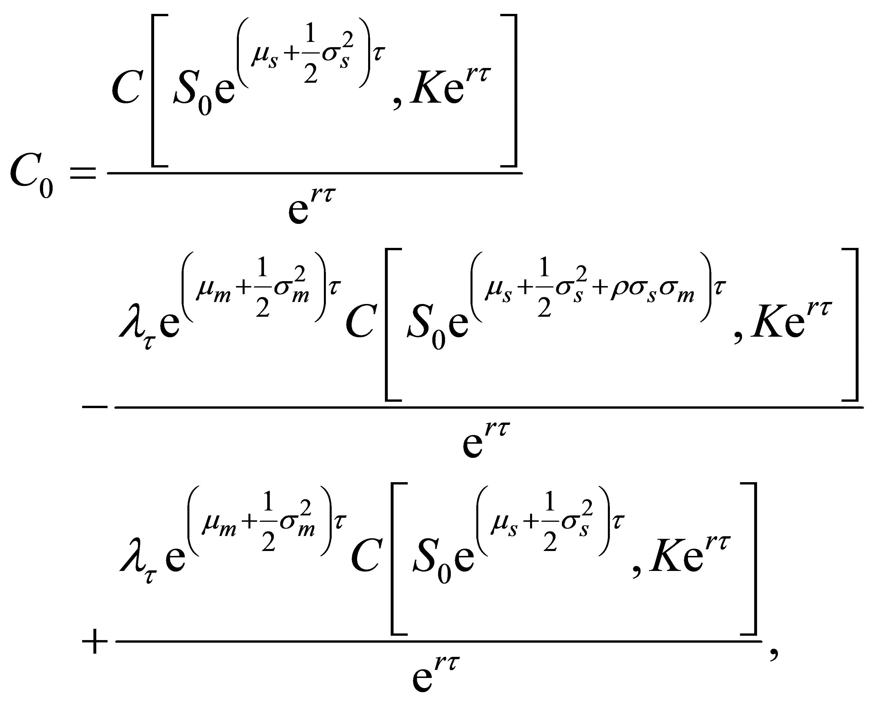
To clearly arrange our analytical results, we use the following notation for the Black-Scholes price of a call with time-to-maturity when the price of the current asset is replaced by and the strike price is replaced by:

(1)

where

In the following, we use some auxiliary variables. Equation (1) will be evaluated for and four different values of,

Accordingly, , , and are used to describe the resulting values of (1). Notice that Equation (1) is linear in and, that is,

3. The Lognormal CAPM in Discrete Time

3.1. Security Market Line in a Lognormal Market

The security market line of the CAPM in discrete time is

(2)

With the given parameters, for a bivariate normal distribution of rates of return on the market, and the underlying asset, both with respect to the holding period, two definitions of are possible. We refer to

(3)

as the asset’s pricing beta, and

(4)

as the asset’s covariance beta2. Note that we define the parameter as the rate of return of the expected value, whereas is also used in the literature to identify the expected rate of return. If the latter definition is preferred, must be replaced with throughout this paper. Of course, since both the asset pricing beta and the covariance beta depend on the expected return of an asset we cannot use (2) to explain returns in a lognormal market. However, setting (3) and (4) equal leads to the lognormal security market line in discrete time. After several conversions, we obtain

(5)

Of course, if (5) holds in the market, an asset’s pricing beta (3) and its covariance beta (4) coincide, and they are equal to one if. In the limit, when the investor’s planning horizon becomes very short, we can apply L’Hôspital’s rule to (3) and (4) to show that

(6)

Therefore, in continuous-time, the security market line (5) is

(7)

the well-known intertemporal CAPM of [8]. However, [9], addressing the relevance of the discrete-time analysis, remarks that “the continuous-time solution is a valid approximation to the discrete-time solution, and its accuracy is a function of the actual structure of returns and the length of the ‘true’ discrete-time interval. I thought to argue for the superiority of discrete-time analysis over the continuous analysis because discrete-time includes continuous time as a limiting case”.

3.2. CAPM Option Pricing in a Lognormal Market

[7] extend the option pricing equations of [2,10], and [11]. In particular, they show that, besides the option’s time-to-maturity, the individual planning horizon is a determinant of an option’s value in discrete time as well. The generalized pricing equations can be presented in terms of the Black-Scholes option values.

For a call option, the certainty equivalent valuation equation of the CAPM is

where

(8)

Here, describes the market price per unit risk for the investor’s planning horizon. In the following, it is assumed that the investor’s planning horizon is shorter than or equal to the time-to-maturity of the option. Then, in a lognormal market, the expected cash flow of a call and the covariance between the cash flows of the call and the standardized return of the market portfolio are3

(9)

(10)

Inserting (9) and (10) into (8) yields the CAPM option pricing model of [7]4,

(11)

In risk-neutral settings,

and Equation (11) equals the call option price of [2].

4. Discrete Option Betas

4.1. An Option’s Pricing Beta

The definition of an option’s asset pricing beta with respect to the holding period is

(12)

Using and (9) results in

(13)

Furthermore, with recourse to (3), (13) yields

(14)

[1,6] derive option betas where the options are evaluated at the Black-Scholes option price (1) and not at the more general CAPM valuation Equation (8), which includes [2] as a special case. Accordingly, to achieve their results, the current call price has to be replaced in (14), Furthermore, the option prices at the end of the holding period also have to be replaced. Thus, we split the option’s time-to-maturity as follows.

(15)

For the remaining period

must apply if the option is evaluated (risk neutral) at the Black-Scholes option price at the end of the holding period. Therefore, , and (14) results in

(16)

Since is linear in and, and

as

applies to the remaining period, (16) yields

(17)

Now, let’s consider two special cases of (17). If the planning horizon becomes very short, we can apply L’Hôspital’s rule and (6) to achieve

(18)

where, if the lognormal security market line (7) holds,

(19)

and is equal to the option’s delta.

Therefore, in continuous time, the beta of an option with respect to the market is given by the beta of its underlying asset times the elasticity of the option price with respect to the stock price. This is a well known result of [1]5.

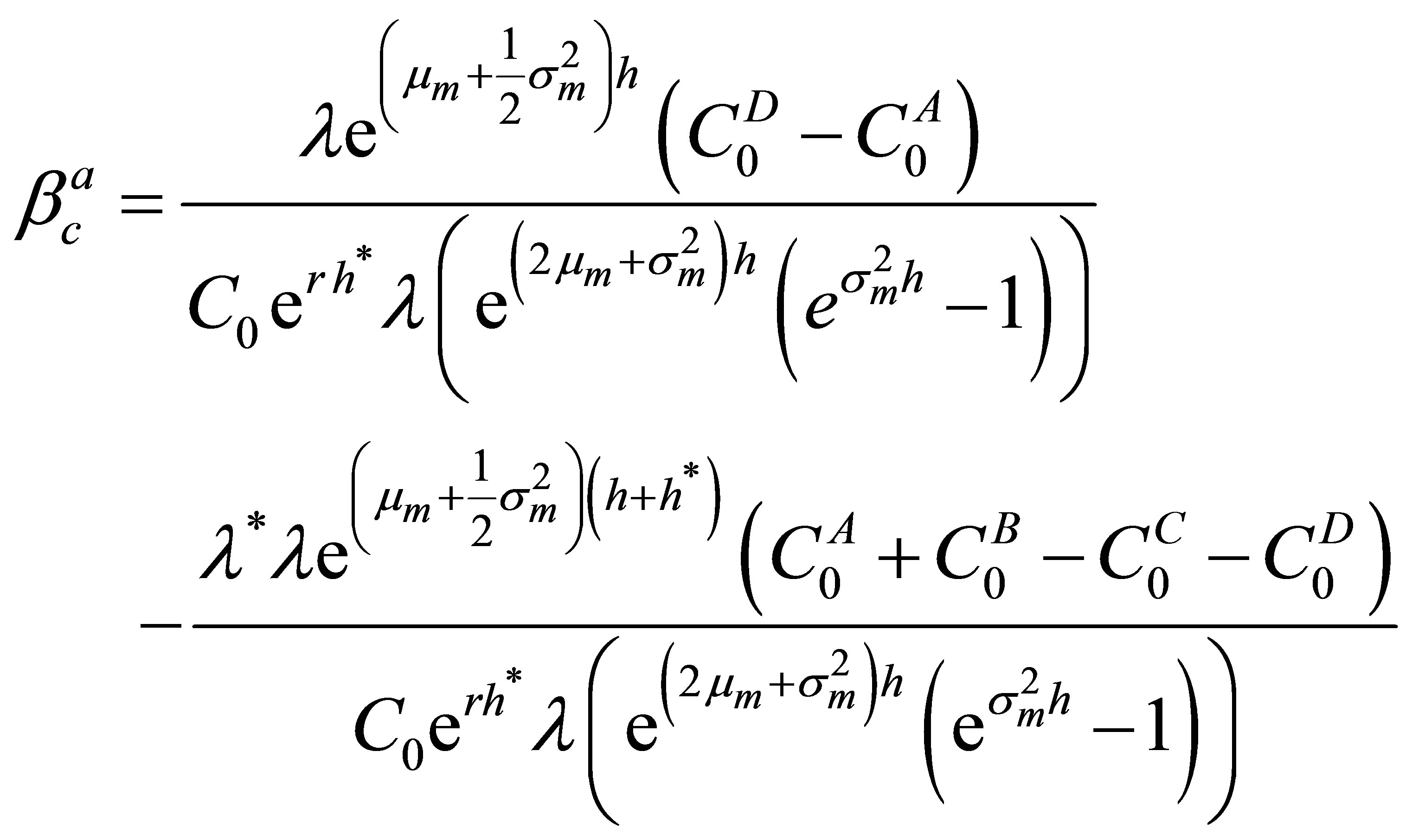
In discrete time, if and the distributions of the rates of return on the market and the underlying asset are bivariate normal, then and. In this case, and (17) is equal to Equation (2.15) of [6],

(20)

who analyze the beta of an option in discrete time with respect to the underlying6. However, if, the bivariate normal distribution of the rates of return on the market and the underlying asset affects both the beta of an option with respect to the underlying and the beta of the underlying, even if options are equal to Black-Scholes prices at the end of the holding period.

4.2. An Option’s Covariance Beta

The definition of the discrete covariance beta is

(21)

where, in a lognormal market,

(22)

Using (10) and (22), (21) is equal to

(23)

Using (4), we can transform (23) to

Using similar arguments as above (L’Hôspital’s rule and (6)), we obtain the special cases, [1]

and [6], Equation (2.10),

4.3. Equality of an Option’s Asset Pricing and Covariance Beta

An option’s asset pricing beta can easily be converted to its covariance beta. Inserting (11) into (13) results in7

Using the definition of in (8) and the definition yields

which is equal to the covariance beta (23). Hence, in contrast to [6], an options’s asset pricing beta and its covariance beta coincide if options are evaluated according to the CAPM option pricing model of [7].

5. Conclusions

Adequate risk measures are essential for both hedging and performance evaluation. This paper extends the option betas presented by [1,6]. Whereas [1] present continuous-time option betas, [6] analyze discrete-time option betas with respect to the stock price and the Black-Scholes option prices. They distinguish between the concepts of a covariance beta, which is based on the covariance between stock and option price changes, and an asset pricing beta, which is related to the option’s expected returns.

We utilize a more general, lognormal option pricing equation, which explicitly incorporates the planning horizon and the investors’ expectations about the development of the underlying asset and the market portfolio, and show how the beta of the underlying asset affects both an options’s covariance beta and its asset pricing beta. Furthermore, the two risk measures coincide if the options are evaluated according to the CAPM option pricing model of [7]. The derived option betas are likely to exhibit a notable economic value. Their utilization might reduce the shortcomings of continuous-time betas applied in empirical studies where the application of discrete-time return measures appears to be more appropriate. Moreover, the option betas are clearly arranged in terms of Black-Scholes option prices and easy to use in practice.

REFERENCES

Appendix A

Definite Normal Integrals

[12] has collected a list of normal integrals, including8

(A1)

where.

To prove the results obtained by [13] and establish the covariance of the cash flow of a CAPM call with the return on the market portfolio, a minor extension of (A1) is required,

(A2)

Proof. Let’s start with the left-hand side. The exponent in (A2) extends to

Using

solves

which also equals the first derivative of the right-hand side of (A2),

Appendix B

Computation of the CAPM Call Option Price

Computation of

When the planning horizon is shorter that the time-to-maturity, we use the results presented by [13] who obtained the expected value of the call for in terms of a Black--Scholes value of an European-style call as9

Furthermore, we take into account that the call option price in a lognormal market for the case can be shown to equal1⁰

where

Thus, we can express the expected value of a call at the end of the holding period as

(B1)

where

(B2)

and

(B3)

are Black-Scholes prices of options with time to maturity of. Splitting (B1) in three integrals and utilizing the solution presented by [13] gives

where

and

Computation of.

We compute the covariance between the value of the call and the return on the market portfolio at the end of the holding period using the decomposition theorem. First, to compute, we must integrate

with and defined as in (B2) and (B3), respectively. Using the definition of the conditional density we obtain the following:

(B4)

Note that the conditional density of the bivariate normal distribution equals the density of the normal distribution with the parameters

such that

(B4) is therefore equal to

(B5)

For the sake of clarity, we first consider only one term of (B5),

(B6)

and split it into two separate components,

(B7)

and

(B8)

We start with (B8). Its exponent

can be transformed into

Next, we make following substitution

Using, (B8) is equal to

(B9)

where

Thus, the integral term of (B9) has the same structure as the left-hand side of (A2). Applying

into (B8) yields

(B10)

Similarly, the exponent of (B7)

can be transformed into

Substituting

and using in (B7) leads to

where

Again, using (A2) yields

such that (B7) takes the following form:

(B11)

Using (B10) and (B11) in (B6) and multiplying by from (B5) gives

The remaining terms in (B5) can be computed in an analogue way such that takes the simple form

where

The covariance is thus given by

NOTES

¹Further empirical studies on option returns which use the Black-  Scholes instantaneous betas are [4,5].

²To calculate the moments of the lognormal distribution, see, e.g., Appendix A in [11].

³The deviation is based on a minor extension of a known integral of the normal distribution, see Appendix A.

⁴A proof of this slightly modified valuation equation is given in Appendix B. A valuation equation for puts and the generalized put betas which follow can be derived in an analogue way. Therefore, the study focuses on call options only.

⁵See [1] p. 190 and p. 210.

⁶Notice that we use the symbol for the holding whereas [6] use. In addition, [6] define the parameter as the rate of return of the expected value, whereas we use it to identify the expected rate of return. To make our results comparable with theirs, the parameter must be replaced with in [6].

⁷Since, we have the term twice in the numerator, with opposite signs and hence cancel them out.

⁸See [12], p. 403, integral 10,010.8.

⁹See Appendix A.

REFERENCES

- J. C. Cox and M. E. Rubinstein, “Options Markets,” Prentice-Hall, Englewood Cliffs, 1985.
- F. Black and M. Scholes, “The Pricing of Options and Corporate Liabilities,” Journal of Political Economy, Vol. 81, No. 3, 1973, pp. 637-654. doi:10.1086/260062
- J. D. Coval and T. Shumway, “Expected Options Returns,” Journal of Finance, Vol. 56, No. 3, 2007, pp. 983-1009. doi:10.1111/0022-1082.00352
- A. Goyal and A. Saretto, “Cross-Section of Option Returns and Volatility,” Journal of Financial Economics, Vol. 94, No. 2, 2009, pp. 310-326. doi:10.1016/j.jfineco.2009.01.001
- S. X. Ni, “Stock Option Returns: A Puzzle,” Working Paper, Hong Kong University of Science and Technology, 2009.
- N. Branger and C. Schlag, “Option Betas: Risk Measures for Options,” International Journal of Theoretical and Applied Finance, Vol. 10, No. 7, 2007, pp. 1137-1157. doi:10.1142/S0219024907004585
- S. Husmann and N. Todorova, “CAPM Option Pricing,” Finance Research Letters, Vol. 8, No. 4, 2011, pp. 213- 219. doi:10.1016/j.frl.2011.03.001
- R. C. Merton, “An Intertemporal Capital Asset Pricing Model,” Econometrica, Vol. 41, No. 5, 1973, pp. 867-887. doi:10.2307/1913811
- R. C. Merton, “Theory of Finance from the Perspective of Continuous Time,” Journal of Financial and Quantitative Analysis, Vol. 10, No. 4, 1975, pp. 659-674. doi:10.2307/2330617
- R. A. Jarrow and D. B. Madan, “Is Mean-Variance Analysis Vacuous: Or Was Beta Still Born?” European Finance Review, Vol. 1, No. 1, 1997, pp. 15-30. doi:10.1023/A:1009779113922
- S. Husmann and A. Stephan, “On Estimating an Asset’s Implicit Beta,” Journal of Futures Markets, Vol. 27, No. 10, 2007, pp. 961-979. doi:10.1002/fut.20285
- D. B. Owen, “A Table of Normal Integrals,” Communications in Statistics—Simulation and Computation, Vol. 9, No. 4, 1980, pp. 389-419. doi:10.1080/03610918008812164
- M. E. Rubinstein, “A Simple Formula for the Expected Rate of Return of an Option over a Finite Holding Period,” Journal of Finance, Vol. 39, No. 5, 1984, pp. 1503-1509. doi:10.1111/j.1540-6261.1984.tb04920.x