Journal of Modern Physics
Vol.08 No.08(2017), Article ID:77882,42 pages
10.4236/jmp.2017.88090
On the Origin of Charge-Asymmetric Matter. III. Properties of Autolocalized Dirac Waveforms
Alexander Makhlin
Rapid Research Inc, Southfield, MI, USA

Copyright © 2017 by author and Scientific Research Publishing Inc.
This work is licensed under the Creative Commons Attribution International License (CC BY 4.0).
http://creativecommons.org/licenses/by/4.0/


Received: June 13, 2017; Accepted: July 22, 2017; Published: July 25, 2017
ABSTRACT
This paper continues the author’s work [1] [2] , where a novel framework of the matter-induced physical geometry was built and an intrinsic nonlinearity of the Dirac equation was discovered. The previous analysis of solitary waveforms’ properties [2] is extended to the four-component Dirac field. It is found that the internal spherical symmetry of the Dirac waveforms is broken to the axial one. The nonlinear Dirac equation is solved and the localized configurations are found analytically. A strict proof that the proper time slowdown is the major mechanism of autolocalization is presented. The previous qualitative conjecture regarding stability or instability of the two types of the waveforms and the origin of cosmological charge asymmetry is supported by detailed analysis. A solution of the problem of mapping between the matter-induced geometry of autolocalized waveforms and the geometry of an ambient Minkowski space is proposed. These results resolve the longstanding puzzle of how the physical Dirac field of real matter becomes a finite-sized particle.
Keywords:
Dirac Field, Affine Geometry, Localization, Cosmological Charge Asymmetry

1. Introduction
In the previous papers of the author [1] [2] a novel framework of the matter- induced affine geometry (MIAG) was developed and the simplest (two-com- ponent) autolocalized solutions of the nonlinear Dirac equations were found in explicit form. The solitary autolocalized Dirac field waveforms in free space turned out to be spherically symmetric, and, most importantly, this symmetry is dynamical; it is a consequence of the equations of motion. Below, we continue our quest for the stationary/stable autolocalized solutions because only these are pertinent to the problem of cosmological charge asymmetry. The requirement of absolute stability seems to be imperative in interstellar or even intergalactic space, but it is not necessarily a prerequisite in laboratory experiments. These are conducted in “normal” charge-asymmetric world with primitive fragments of antimatter created artificially, and then thoroughly guarded in sophisticated traps.
The Problem. In this study, we aim at finding solitary static autolocalized solutions of the Dirac equation along with a proof that the generic nonlinear mechanism of autolocalization (the local time slowdown) favors matter over antimatter. From this perspective, the case of hydrogen or anti-hydrogen atoms is not a one-body problem, and it is not addressed here. Autolocalization of the Dirac field from fluctuations in a uniform background (which will be addressed in another paper) is most likely a very slow and rare transient process that ends up with a proton. Its timescale and relative weight of all the underlying processes and/or mechanisms are not yet clear, but the Universe definitely had enough time to conduct such an experiment. Unlike the pioneer work by A. Sakharov [3] , where the origin of currently observed charge asymmetry was attributed to the violation of CP-invariance and nonequilibrium processes in the early hot Universe, this work ascribes it to the fundamental mechanism of the Dirac field autolocalization.
The present work extends the previous results [2] to a more realistic case of the four-component Dirac field. Being otherwise unwieldy, calculations are significantly simplified by accounting, ab initio, for the earlier discovered [1] dynamical spherical symmetry; below, we call it the “spherical ansatz”. The explicit calculations confirm our previous conjecture that only one of the two major types of isolated localized solutions is genuinely stable (has well-defined energy and satisfies all the consistency conditions). It is identified as a particle with positive charge and negative energy. It is imperative to find, as the next step, the transient process that ends up with a stable autolocalized waveform.
The Method. The earlier developed [1] mathematical background for the present work is based on the following ideas and results. It has been observed long ago [4] that if a physical Dirac field is defined at a point in spacetime continuum (the principal differentiable manifold ), then such field deter- mines the tetrad of Dirac currents. These are linearly independent and Lorentz- orthogonal. They can serve as local algebraic basis for any four-dimensional vector space, including the infinitesimal displacements in coordinate space. The singular case when the Dirac currents are lightlike, which is possible only on a two-dimensional surface in spacetime, is not considered here. With this excep- tion, the Dirac field provides the means to navigate through the spacetime so that geometry can be viewed a descendant of stable Dirac matter.
The Dirac currents (one timelike and three spacelike) are further employed as the Cartan’s moving frame in spacetime, which, in its turn, resulted in the technique of covariant derivatives for the vector and spinor fields. The physics was naturally brought into this mathematical picture by the equations of motion of the Dirac field. The 28 primary differential identities that were derived in [1] from equations of motion fully determined all the components of the matter- induced affine connection (the Ricci coefficients of rotation of the tetrad) in  and without resorting to a particular coordinate system. Connections determi- ned this way completely defined an affine geometry (endowed with the connec- tion but with no metric), which was dubbed [1] a matter-induced affine geometry. With known connections, it became possible to find the coordinate lines and surfaces of the MIAG, all of which have a clear physical meaning and quite high degree of symmetry. Notably, the MIAG uniquely determines the hypersurfaces of constant world time of a waveform, though inside a stable solitary waveform there can be neither events nor propagating signals (not to speak of rods and synchronized clocks)1.
The general properties of coordinate surfaces in  are discovered in [1] without any assumptions regarding the nature of an ambient space or the Dirac field. It appears that the main qualitative characteristic of the stationary Dirac object is the direction of axial current, which can point only outward or inward. It was realized that the locally defined notions of outward and inward are prerequisites for any reasonable discussion of the localization phenomenon. The framework of matter-induced affine geometry not only ideally fits this goal but also explains the autolocalization, as it is seen in the real world, as an intrinsic property of the Dirac field. For a waveform with the mass parameter m, the nonlinearity of Dirac equation is effective at distances comparable with the Compton wavelength,
 .
.
The Outline and Results. The paper is organized as follows. Section 2 provides a concise overview of the results of the author’s papers [1] and [2] , where the concept of MIAG was introduced. In Section 3.1 we explicitly translate the previously established spherical symmetry into the requirement that the axial current only have one nonzero component . The spherical ansatz carries no ambiguity, since the congruence of lines of the axial current is both normal and geodetic. Section 3.2 accumulates observations from a frontal attack on the nonlinear system of equations for the four-component Dirac spinors, which point to the most rational choice of variables. At the end of this section we describe the complete protocol of mapping the ambient space
  onto physical manifold
 , where all “geometric quantities” are defined by the Dirac field. The radial coordinate r, which is compatible with the matter-defined affine curvature and can serve as a usual coordinate in the ambient
 , is introduced in Section 3.3. The 16 additional differential identities (this time, for the convection currents), that serve as a test for the stability of the solitary waveforms are derived in Section 4. Using the “optimal variables” found in Section 3.2, the original system (written down explicitly in Appendix B) is reduced to the real-valued equations in Section 6, which are thoroughly analyzed in Section 0 for
  and in Section 7 for
 . The analytic solutions in natural variables of the physical manifold
  are found in Section 6.3. Here, we find more evidence that the mode
  is unstable. This issue cannot be resolved within a one-body problem. Essentially, for both modes the vacuum level
  follows from equations of motion and it cannot be altered by a fiat.
The analytic solutions in variables of the ambient space  are found in Section 7.2. When the energy of a waveform is defined with respect to the world time
  of the ambient Minkowski space, then there is no way to resolve the proper time slowdown. There is no difference between the shapes of
  and
and ; the vacuum level of invariant density for both modes appears to be
 . Furthermore, their shape is not fixed any by the nonlinear dynamics (as it should be for all autolocalized waveforms, e.g. solitons). This is an ultimate proof of the previous conjecture that proper time slowdown is the major mechanism behind autolocalization in physical manifold
 .
.
The last section points to several intriguing results which did no receive the discussion they deserve. All of them are challenges that could not be addressed in this paper, because they probably cannot be met within the scope of one-body problem. We are just making physically motivated conjectures. For example, we propose to look for a correlation between the excess of positrons in cosmic rays and strength of magnetic fields in their sources.
2. The Framework
Looking for a solution of the practical problem of autolocalization of the Dirac field into solitary waveforms I proposed a novel concept of matter-induced affine geometry (MIAG) [1] . It stems from the observation that Dirac field , being a coordinate scalar, naturally generates at a point
  an affine centered vector space (spanned by the Dirac currents), which is similar to the tangent space
  of the four-dimensional manifold
  (spanned by the vectors
  or
or ). It determines, at any point
  of spacetime, a locally Minkowskian basis comprised of four Dirac currents
  defined on the principal physical manifold
 . These are the vector current
 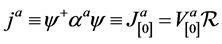 , the axial current
 , and the two “charged currents”, which are the real and imaginary parts of the
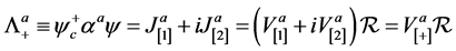 . Here,
  is the invariant density of the Dirac field. The latter is defined as
 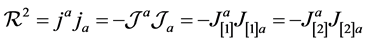 , which is small subset of many Fierz identities [5] , and, by definition,
 . The superscripts
  numerate the Dirac matrices and also the components of the Dirac currents with respect to tetrad basis
  , which belongs to an “intermediate” manifold
 . By means of yet another Fierz identity, viz.
 (2.1)
(2.1)
where  is a usual pseudo-Euclidean Minkowski metric, the quadruples
 ,
,  , form a complete set of orthogonal unit vectors (even though no notion of length has been introduced). The quadruple
  is the solution of the linear system,
 . Therefore, all indices are moved up and down by the Minkowski
  or
or , which is nothing but a consequence of the Fierz identities2. The quantities
  and
and  are the scalar and pseudoscalar densities, respectively, and
 . Expressions for the Dirac currents and scalars in terms of ampli- tudes and phases of the Dirac field’s components are presented in Appendix A.
The covariant derivative of the Dirac field is of a standard form,  . It is determined without leaving the principal manifold
 . The connections
  of the Dirac field are
 (2.2)
(2.2)
in tetrad basis  of principal manifold
  and in auxiliary basis
 , respectively. We adopted, without discussion, the usual Dirac equations of motion in these bases,
 (2.3)
(2.3)
with an arbitrary mass parameter m. Using the Dirac currents as a moving frame, we explored differential identities for the curls and divergences of all four Dirac currents and found all components of the affine connection  (the coefficients of rotation of the tetrad). The nonzero elements of the
  in the tetrad basis of the normalized Dirac currents
  are as follows:
 (2.4)
(2.4)
where  is the derivative of invariant density
  in direction of the axial current, and it has an algebraic representation via the pseudoscalar density
 . Hence, the equation of motion (2.3) acquires a term, which is linear in Dirac field
  and in pseudoscalar
 , which, in its turn, is bilinear in
 . Therefore, Dirac equation becomes a nonlinear system,
 (2.5)
(2.5)
where the anomalous term,  , singles out the direction of axial current among others even when an external field
 . The notation
  discerns between the cases of outward and inward directions of the axial current of the localized Dirac waveform, which must be considered separately. In the first case
 , and in the second case
 , where
  is the “natural” tetrad component of the vector potential in the connection (2.2). This difference came from the requirement that the radial coordinate, as measured along the congruence of axial current, increases in the outward direction. The Dirac matrix
  (a.k.a.
 ) differentiates between the right and left components, and it stands for +1 for
  and for −1 for
 .
.
The dynamics of the Dirac currents determines, in a unique way, the hypersurfaces of constant world time  and of constant radius
  in
in ;
;  and
and  are the natural parameters along normal congruences of vector and axial currents, respectively. Because the differentials
  and
and  are complete (integrable), both
  and
and  are the matter-defined holonomic coordinates over
 .
.
Coefficients  of rotation of the tetrad basis are determined within the principal manifold
 , which guarantees that nothing in
  depends on the choice of coordinates in arithmetic
 . The analytic two-component solutions of the nonlinear Dirac equation (2.5), which were found in Ref. [2] , in absence of external electromagnetic field, are of two types. One of them,
  , has the directed outward (or up) axial current and a magnified invariant density,
  , in its interior. There, the proper time
  flows slower than the world time
  (which is the same across the entire waveform). These waveforms are supposed to be small, heavy, and positively charged particles. Waveforms of the second type,
  , with the axial current directed inward (or down), have a reduced invariant density,
  , in their interior, so that the proper time flows faster than the world time. They must be light, negatively charged, and cannot be truly localized or even stationary unless there exists an external “attractive field”; otherwise, waves of the Dirac field will tend to escape into ambient space.
Since  and
and , these two directional derivatives yield two additional nonlinear terms to the Dirac equation (2.5). The first of them is solely responsible for the local time slowdown, which gives a major contribution to autolocalization. In fact, this is the main physical mechanism behind autoloca- lization of any wave field, which always tend to concentrate in domains with the minimal phase velocity.
In this paper, we consider the general case of four-component Dirac spinors and address the issue of stability more thoroughly. Namely, we examine whether the autolocalized Dirac waveforms, which were discovered within the MIAG framework, satisfy an extended set of differential identities (unconditionally or under specific conditions). For some of them, the answer will be affirmative. These are the true physical solutions. All others must be rejected. In a sense, the additional identities play the same role as boundary conditions that can validate or invalidate certain solutions as being pertinent to a physical problem. To derive them, we will also need the Dirac tensors,
 (2.6)
(2.6)
where  stands for a skew-symmetric product. These tensors satisfy the following Fierz identities, which allow one to express them via vectors and scalars [5] ,
 (2.7)
(2.7)
where . Mathematically, because the covariant derivatives of the tetrad vectors are just the coefficients of rotation,
  , it will be easy to calculate the derivatives of these tensors.
3. The Four-Component Dirac Spinors, Qualitatively
Below, we explore the properties of the four-component solutions. In this paper, advancement became possible due to the following earlier observation. Three of four Dirac currents (the vector current,  , and two charged currents,
 ) constitute a canonical system with respect to the congruence of axial current
  [1] 3. Therefore the entire tetrad is Fermi-transported along the lines of vector field
 . These lines point into radial direction, and their congruence appears to be both normal and geodesic over the principal manifold
 .
.
3.1. Spherical Ansatz
An oddity of the Dirac field is that it cannot be embedded into an arbitrary coordinate background, just because establishing of relation between the internal basis of the Dirac currents in the principal manifold  and the ambient coordinate space
  requires three tetrads, viz.,
  , the tetrad
  and a judicially chosen “coordinate tetrad”
  (e.g. of rectilinear or spherical coordinates.). They are interrelated by means of an a priori unknown Dirac field. Only coordinates
  must be totally arbitrary (the physical Dirac field is a coordinate scalar).
Parameter  on the radial geodesic (which is not an affine parameter) is a holonomic variable, i.e., the radial coordinate
  is well-defined4. The vectors of geodesic curvature of the lines of other three currents,
  ,
,  , and
, and , have the same normal component as the mean curvature vector of the umbilical surface
  (of constant
  and
and ) and hypersurface
  (of constant
 ). As a result, all three currents passing in a tangent direction through a point on hypersurface
  of a given radius
  never leave this surface (see Ref. [1] , Section 6). These facts clearly point to a possibility that Dirac equation (2.5) can have solutions where axial current has only one component,
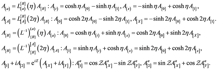
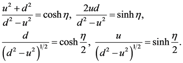
 . Then, orthogonality of the tetrad requires that
 . Inspecting Eqs. (A.4) and (A.5), we readily find that left and right amplitudes must be equal (since
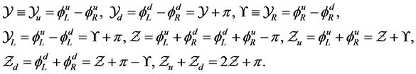
 ). The sums of the phases,
  and
and , in their turn, must differ by
  (since
 ),
),
 (3.1)
(3.1)
Within this ansatz, the most general expressions (A.4)-(A.5) for the Dirac currents simplify to
 (3.2)
(3.2)
The scalars ,
,  and
and  (cf. Eqs. (A.6)) simplify to
Below is the list of notation and useful identities that stem from the ansatz (3.1) and will be extensively used:
 (3.3)
(3.3)
It was established earlier [1] that within any connected domain where  we have
 (3.4)
(3.4)
i.e., that these quantities depend only on holonomic radial coordinate . When
 , the spatial triad
  with
with ,
,  is right-handed and axial current
  is naturally directed outward, i.e.
 . When
 , the latter is directed inward, but if we still wish
  to point outward, then we have to take
 ,
,  ,
, . These two cases must be treated separately.
3.2. Tetrads Induced by Nonlinear Dirac Equation.
This section is a blueprint for Appendix B and Section 5, where the nonlinear Dirac equation (2.5) is reduced to a solvable form. In a nutshell, it presents an overview of a sequence of transformations of variables that allow for a streamlin- ing of the otherwise excessively laborious calculations. It also provides a deeper insight into dynamics of localization from the perspective of ambient space.
It is impossible to find an explicit analytic or numerical solution of the Dirac equation without specifying a coordinate basis in  and a basis of the Dirac matrices. Here, as in Ref. [2] , we employ the numerical matrices
  in spinor representation (A.2), and associate them with a tetrad
 . Then, the Dirac matrices of Eq. (2.5) are
  (see Section 3 of Ref. [2] for the details), while the directional derivatives
  remain in the basis
 , which is associated with coordinate lines and surfaces [1] determined in the principal manifold
 . In this mixed representation, Dirac equation reads as
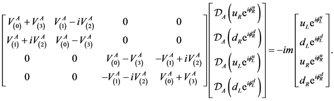 (3.5)
(3.5)
The operators , which are copied from Eq. (2.5), are as follows,
 (3.6)
(3.6)
Since , it is helpful to assemble the operator,
  . The coefficients
  , which are read out from the ansatz (3.2), are as follows,
 (3.7)
(3.7)
The rest of this section is based on the observations made in the course of straightforward, lengthy and tedious calculations based on direct use of the coefficients (3.7). The latter can be significantly simplified. Let us use the second Eqs. (3.3) and trade  and
and  from Eqs. (3.2) and (3.7) for
  and
and . Then, the second line of Eqs. (3.7) can be identically rewritten as
 (3.8)
(3.8)
Just by inspection, one can observe that after expressions (3.8) are substituted into the original system (3.5), the derivatives  and
and  in the directions
  appear only in the combinations
  and
and . Therefore, the currents
  and
and  can be
traded for their combinations,  and
and  , which is instructive to cast as
  . The new tetrad,
  , where
  and
and  numerate vectors and their components, respectively, reads as
 (3.9)
(3.9)
The currents  and
and  of the tetrad (3.2) depend only on sums of two phases, so that they rapidly oscillate with the “world time”
 . The components of all currents (3.9) depend only on the difference
  and do not depend on
 . Obviously, the quadruples
where , comprise a new tetrad, which is completely equivalent to the original one, and it satisfies the same conditions (2.1) of ortho- gonality and completeness. Its vectors point into principal “angular directions”
 on a spherical surface
  spanned by the streamlines of the vectors
 . In this new basis, the primary tangent tetrad vectors
and coefficients  are
are
 (3.10)
In order to make explicit (or even numerical) calculations possible, the objects defined on  must be embedded into coordinate
 . To begin with, one has to choose a particular tetrad
  numerated by subscript
  (the same one that numerates rows in (3.2) and (3.9)) and project the derivatives in directions of tetrad (3.9) onto the basis
  5, i.e.,
 (3.11)
These equations contain derivatives  only in the combinations
  and
and , where
 . Therefore, the original tetrad vectors
  can be traded for their combinations,
  ,
,  , or simply
 .
.
This trade-off is nothing but the result of rotation of the basis  by an angle
  around radial direction
  (or, equivalently, around
 )6. In terms of the new tetrad,
 :
: , one can rewrite (3.11) in a compact form as
 (3.12)
where the “tangent rapidity”  depends only on the ratio
 ; it is intro- duced in such a way that
  and
and . There- fore, the natural counterpart of the tetrad
 ,
,  is the tetrad
 ,
, . Now, visually evaluating the result of straightforward calculations (explicitly given by Eqs. (B.2) and (B.9)), which employed the tetrad (3.2), one can see that the derivatives
  of the components
  of the Dirac spinor consistently appear only as linear combina- tions,
 (3.13)
Transformations (3.12) and (3.13) of the directional derivatives correspond to the following transformations of the tetrad vectors:

 (3.14)
Since transformations (3.14.a) and (3.14.b) are reciprocal, we find that the tetrad  is completely determined by the Dirac field
 ,
,
 (3.15)
Hence, we can identify the tetrad directions  of (3.14.b) with the directions
  of (3.14.a). Then,
  ,
, . It is clear that
 , i.e. that the tetrad
  is not an object from the coordinate manifold
 .
.
Transformations (3.14) engage only temporal and azimuth directions, ( and
and ). Therefore, for the four-component Dirac field, the
  appears to be the direct product of the two-dimensional subspaces
  (and not
 , as it was for the two-component spinors). One must keep in mind that
  and
and  are the only holonomic (i.e. well-defined) variables, so that the integrals
  and
and  between two points do not depend on the integration path7. The angular variables
  and
and  (and, accordingly,
  and
and ) are non-holonomic. The intermediate variables
  and
and , which mix holonomic
  and non-holono- mic
 , are non-holonomic also.
The main result of the foregoing qualitative analysis is that the following string of transformations,
 (3.16)
reduces the matter induced tetrad to a surprisingly simple system of unit vectors,  at a point
 ,
,
 3.17)
3.17)
In this new basis, the Dirac currents become
 (3.18)
Remarkably, in this representation, the new tetrad vectors depend only on amplitudes, but not on phases of the components of the Dirac spinor. When either  or
or , Eqs. (3.16) reproduce tetrad vectors used in Ref. [2] for the outward-or inward-polarized two-component solutions
  and
and , res- pectively.
Once a solution of the Dirac equation is found, i.e., the parameters ,
,  and
and  of the transformations (3.15) are known, one can view
  as a dynamic mapping of the Minkowski
 . As a matter of fact, the basis (3.17) is a locally pseudo-Euclidean tetrad
  subjected to the non-unitary Lorentz-like transform
  with velocity
 , within the azimuthal
  -tangent plane,
 (3.19)
where  are the tetrad indices in differentiable manifold
 , endowed with spherical coordinates in Minkowski space. It should be noted, that the matrices
  and
and , are not tensors and that their indices even belong to different spaces. They just happen to share the same parameter
  of Lorentz- like transformations.
Strictly speaking, in the framework of the matter-induced affine geometry (MIAG), we are dealing not with the locus of points equidistant from a center, but with the so-called affine sphere, for which all affine normals intersect in a single point. The MIAG naturally yields the mean curvature of the umbilical submanifold  as a function of the Dirac field,
 . But it would be incorrect to claim that the radius of curvature is the inverse of H,
  , simply because length is not even defined within the affine geometry. At best, one can have a parameter that orders points along each particular curve. In can actually be checked in a straightforward way that for the previously found explicit solutions [2] ,
 . The character of this inconsistency prompts a pragmatic (or just a poor man’s) solution.
Since the congruence of lines of the vector  is normal and geodesic, one may start with the technically simplest choice of
  as radial coordinate of point
  (or, alternatively, the affine parameter
  along it), and attempt to find such a radial variable
 , that the mean curvature
 . Thus introduced variable
  is the radial distance compatible with the affine curvature
 . Then, if
  is the area of sphere passing through point
 , we will have the accustomed relation,
 (3.20)
In order to proceed, we have to specify a coordinate system  with the components
 , endow it with the tetrad
  and map the ambient
  onto inner
 . The corresponding procedure is fairly simple. One must start with Minkowski space and choose there a sphere of radius
  endowed with spherical coordinate net
  and tangent vectors
 . Next, consider at any point
  of this sphere the vectors
  in temporal and azimuthal directions. Then perform Lorentz boost
  in the
  plane, which, according to (3.19), will transform the tangent vectors
  into the couple
 . The second boost
  in the same plane will transform, according to (3.14.a), the vectors
  into
into  of the principal manifold
 . Overall the entire mapping
  is just the boost
 , where
  for
for  and
and  for
for . Then, according to (3.19) and (3.14.a),
 (3.21)
Similar relations hold for the directional derivatives in the same bases, i.e., we can replace in these equations  while preserving the same indices. In Section 5 we will find that equations of motion require that
  and
and . Therefore the time-dependent components
  and
and  are the result of transformation of the time-independent
  into local frame, which is rotating with the angular frequency
  8.
8.
3.3. Discussion and Outlook
It must be clearly understood that none of the transformations of the Dirac currents from their original form (3.2) to (3.9) and, ultimately, to (3.17) and (3.19) affect the Dirac field of a wave form, which is a coordinate scalar. Each one of the transformations (3.16) is a mapping between equivalent tetrads at a point . The parameters of these local transformations,
  ,
,  and
and , are completely determined by a yet to be found solution
  of the Dirac equation (3.5). None of them (as will be shown below) depends on the radial variable
 . As anticipated, dynamic of localization appears to be strictly internal and local.
1) Spherical symmetry. Three manifolds, the physical , the intermediate
 , and even arithmetic
  share the same radial geodesic lines [1] . None of the transformations (3.16) depend on their parameterization. The holonomic radial coordinate
 , the affine parameter
 , or any
  are equally good parameters (cf. footnote4). Most importantly, the hypersurface
  of a constant radial parameter and the surface
  of constant
  and world time
  are the umbilical submanifolds of
  9. The two-dimensional umbilical submanifold
  of a constant positive mean curvature is an ordinary sphere [8] [9] .
Our immediate goal is to match the two coordinate systems. One of them,  is associated with the local tetrad
 . Here,
  and
and  are the lengths of azimuthal and meri- dional arcs, respectively, on the 2-d sphere of radius
 . The second one is a particular (preferred) system of the rectilinear coordinates of Minkowski space,
  , which are expressed in terms of oblique spherical coordinates. One can say that the system
  interpolates between
  and
and , provided the polar axis
  is fixed with respect to the rectilinear coordinates
  by the same angles
  and
and . In a sense, the spherical symmetry of the ambient space
  is matter-induced by the internal physical space
  of a solitary localized waveform. Just by a visual comparison, it is clear that for any fixed polar angle
  the line of the matter-defined coordinate
  is confined to the 2-d plane
  spanned by the coordinates
  and
and , which is parameterized in polar coordinates by the same angle
  as the line of coordinate
 . Therefore, in three dimensional space, the normal vector to this plane is parallel to the axis
 ; this vector can be naturally associated either with the 3-d spin of the waveform or an “axis of quantization”, or a kind of “orbital motion” around the polar axis
 . The
. The  component of the vector potential, even if it is a (nonzero) constant, leads to a finite circulation of
  over a closed contour laying in the 2-d plane
 . Hence, there is a finite flux of an external magnetic field along
 . In a most startling way, the MIAG leads (or could have led) to the prediction of a magnetic moment of the localized Dirac waveform.
Though in the primary (algebraically defined) basis  of the Dirac currents (3.2) the dynamical spherical symmetry is perfect, it is dynamically broken in the bases
  (3.17), which are induced by the solutions of the equations of motion (3.5). The spherical symmetry of the ambient space
  remains unbroken. These are precisely the rectilinear Minkowski coordinates
 , where the points are normally associated with events10, that can be subjected to the uniform Lorentz transformations and/or rotations in the ambient
 , while all physical quantities, including the axis of quantization of angular momentum, that have their primary definition in
  are the coordi- nate scalars. Transition to the coordinates
  is also a first step towards the problem of a moving waveform as well as of two waveforms/bodies.
2) Radius of a sphere. As it was just mentioned, the radial variable  is poorly suited for this purpose just because the geodesic curvature
  on the principal manifold
 . Furthermore, the curvature
  reaches its maximum not at the supposed geometric center
 , but at the distance
 , the inflection point of the curve
 . It normally approaches zero when
 , and it does the same abnormally when
 . Therefore, “radius”
  does not match the curvature
  in a usual geometric sense. Since the radial lines are geodesic (and literally straight), it is possible to find such a compatible with the matter-induced curvature radial variable
 , that
  (and Gaussian curvature
 ). This means that for a solitary Dirac waveform the phase difference,
  (as well as the scalars
 ,
,  ,
, ), can also serve as a measure of the distance in radial direc- tion. For the two-component mode
  the function
  was found in Ref. [2] . It appears to be exactly the same for the four-component mode
 , though its derivation is much more intricate (see Eqs. (6.24) with
 ),
),
 (3.22)
Hence, the variable  does not cover the domain
 ;
; . The inverse function is double-valued,
 (3.23)
where the upper and lower signs correspond to the “exterior” ( ) and “interior” (
 ) of the waveform, respectively. For both bran- ches,
  , but
, but , while
 . In other words, in terms of radius
 , the point
  becomes infinitely remote. Interestingly enough,
  at the inflection point
  of the function
  (the point where
 ). We will continue this discussion in Section 6, after we find the explicit solutions fo both
  - and
- and  -modes.
4. Differential Identities for Convection Currents
Equations (2.5) with the coefficients of rotation (2.4) are descendants of the nonlinear Dirac system (2.3). These equations incorporate only the same 28 differential identities that were derived in Ref. [1] and completely determine the geometry of the Dirac field of the solitary waveforms. Since these identities are derived from the equations of motion, the properties of the waveforms found so far (like being stationary and spherically symmetric) are the dynamic symme- tries. However, not all solutions of these equations are physically acceptable. Of the two two-component analytic solutions found in Ref. [2] , only one is unques- tionably stable, which indicates that, possibly, not all relevant constrains were found and/or employed. In this section, we derive more identities that fill in these blanks.
The well-known Gordon’s decomposition of the vector current  is one more differential identity that follows from the Dirac equation of motion. It aims at a qualitative dissecting of the vector current into flux of electric charge (bulk motion of localized charged particles, usually dubbed as convection/conduction current) and local electromagnetic polarization (e.g., proper or induced electric and magnetic moments) frozen into this flux. After the bulk transport is separated, the internal dynamics of a localized waveform is encoded in polariza- tion tensors (2.4). In classical electrodynamics, charged particles are considered pointlike and governed by ordinary differential equations of their trajectories. A gap with continuous nature of field described by PDE has never been consis- tently bridged, mostly because an intrinsic mechanism for localization of a realistic field of a matter has not been found until recently [1] [2] .
Originally, the Gordon’s decomposition was introduced as an identity for the vector current, in which transport and polarization parts are explicitly split. Here, we are dealing with four Dirac currents, and each of them allows for such decomposition. The procedure and result appear to be very similar for the Dirac currents ,
,  , and
, and . For the axial current
 , the result is even qua- litatively different, but it prompts more useful identities involving fluxes. Flux of the pseudoscalar density,
  is of special interest for the unstable mode
 , since its decay must result in additional “propagating waveforms”. Overall, the Gordon decompositions of the Dirac currents provide 16 differential identities that must be satisfied for stable solitary waveforms. While we have no compre- hensive approach, a picture of fluxes in ambient space
  seems to be the only way to learn what the products of decay can be.
1) The vector current . The Gordon’s decomposition of the vector current is readily obtained by replacing
  and then
  in the definition
  with the r.h.s. of the Dirac equation (2.2) and its conjugate, viz.,

After taking the half-sum and splitting the products of Dirac matrices as  the result reads as follows:
 (4.1)
(4.1)
and, as long as  satisfies equations of motion (is an on-mass-shell solution), this is just yet another identity. By virtue of (2.1), the expression in brackets in second term becomes
 , so that (c.f. Eq. (2.6))
 (4.2)
(4.2)
In holonomic coordinate basis, this would be a well-known result. To com- pute , we resort to the Fierz identity (2.7.a). Using the previously found coefficients of rotation, Eqs. (2.3), we find that the second term in (2.7.a) does not contribute to
  and
and
 (4.3)
(4.3)
Collecting all terms proportional to  in the l.h.s., we obtain the final result for the convection flux of the scalar density
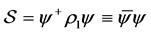 ,
,
 (4.4)
(4.4)
which differs from the commonly known in three respects. First, only the current of unstable mode , where
 , is affected by the electro- magnetic field. Secondly, the directions of convection and total currents do not necessarily coincide. Third, for stable mode
 , where
 , the convec- tion part in the r.h.s. of the last equation differs from total vector current
  only by a scalar factor
 , so that convection and total currents are parallel (which hints an intrinsic stability). Finally, one can determine the fraction of polarization current within the total one in both modes.
2) The axial current . The Gordon’s decomposition of the axial current is surprisingly different. Since
  and
and  we can rewrite the axial current in two ways,
 (4.5)
(4.5)
Taking the half-sum of these two expressions and separating symmetric and skew-symmetric products of Dirac matrices, we obtain
 (4.6)
(4.6)
Unlike the previous case, we find in the axial current neither convection flux, nor a recognizable polarization component. Instead, the last equations allows one to discover that the pseudoscalar density  of the Dirac field has the intrinsic property of propagation and can be viewed as a relativistic field in its own right [10] .
The expected pattern of the convection current of the pseudoscalar density emerges if, instead of the sum, we take difference of the substitutions (4.5). This results in an identity,
 (4.7)
(4.7)
which looks similar to Eq. (4.10), except that there is no full axial current in its l.h.s. Proceeding as previously, we find that the second term in (2.7.b) does not contribute to  and
and
 (4.8)
(4.8)
Therefore, the convection current of the pseudoscalar density 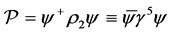 does exist and is as follows:
 (4.9)
(4.9)
Quite understandably, the pseudoscalar density is carried not by a spacelike axial current,  , but by a timelike vector current,
 .
.
3) The “charged currents” . The Gordon’s decomposition of the charged currents employs two representations,

This case is very similar to the first one, and the result
 (4.10)
is similar to (4.2). There is no counterpart to the second term of Eq. (4.2) here simply because , which is one of the Fierz identities [5] . The r.h.s. of Eq. (4.10) can be computed using the Fierz identity (2.7.c). Since the Dirac current
  is complex-valued and thus gauge variant (unlike the real currents
  and
and ), its gauge-invariant covariant derivative consists of two parts,
 . Accordingly,
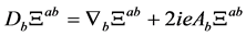 . Once again, using Eqs. (2.3) and exercising some algebra we obtain,
 (4.11)
and rearrange Eq. (4.10) as
 (4.12)
with the same observations as for Eq. (4.4). Putting here for  its explicit representation (2.7.c) we obtain
 (4.13)
where  and the tetrad index of the basis
  can be replaced by any other tetrad index, including the coordinate index
 . In the last equation, the component
  of the vector potential can be eliminated by a gauge transformation (c.f. footnote11). For the convection part of the charged current (A.8) in the l.h.s. of (4.13) to be nonzero, the Dirac field of a waveform must have both
  and
and  components, which is not required in the r.h.s.
It should be noted that the density, corresponding to the convection current (4.13), is zero, which is just one of many the Fierz identities, . The physical meaning of this current is unclear and we will refrain from using this equation as an additional constraint.
5. The Four-Component Dirac Spinors. Reduction to Real-Valued Equations
In this section,which is mostly technical, we carry out the program outlined in Section 3.2. The cases  and
and  are considered separately. They belong to the different spacetime domains separated by a singular two-dimen- sional surface
 , where all four Dirac currents become lightlike. The question that remains open is whether these domains can be parts of a single solitary waveform. We begin with reduction of the system (3.5), which is written down in expanded form in Appendix B, to real-valued equations. Subsequent analysis drastically simplifies the coordinate dependencies, so that we end up with the system of ODE.
The differences of first equations in couples (B.4.a)-(B.5.a) and in (B.11.a)- (B.12.a) yield the expected general result,  , well known as a non- conservation of the axial current. Namely,
 (5.1)
(5.1)
where, we remind,  ,
,  and
and  (cf. Eq. (3.1)). In fact, these phase differences determine the shape of waveforms, which is rather a rule than exception for autolocalized solitary solutions of all wave fields.
The sums of Eqs. (B.4.a)-(B.5.a) and (B.11.a)-(B.12.a), after using Eqs. (5.1) to exclude 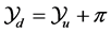 and exercising simple algebra, result in
 (5.2)
(5.2)
where the box emphasizes results, which will be used later without a notice (especially in lengthy equations). Hence, away from a singular surface , the rapidity
  in tetrad (3.17) does not change in radial direction, making invariant density
  and phase differences
  the only r-dependent functions.
In Eqs. (B.4.a)-(B.5.a) and in (B.11.a)-(B.12.a), like , one can safely put
 . Therefore, the sums of phases,
  and
and , do not depend on radial variable
  either. (As a matter of fact, neither
 , nor
, nor  show up in any of the equations below11.) But according to (3.1) and (3.3), we have
 . Therefore,
  is also r-independent. Finally, the phase differences
  and
and  obviously do not depend on
 . Recalling Eqs. (3.4), we conclude that the only r-dependent phase differences are
  and
and . It is also clear that the ratio
  (when
(when ) (or
) (or , (when
 )) also does not depend on
 . These observations lay firm ground for the future separation of radial variable
  in equations that determine localization.
Analysis of the Eqs. (B.6), (B.7) and (B.13), (B.14) is more cumbersome, and the cases of  and
and  will be analyzed one-by-one.
1) The  -mode,
 .
.
Let us multiply Eqs. (B.6) and (B.7) by  and
and , respectively, add them up, and divide the result by
 . Next, we make the following substitutions:
 (5.3)
(5.3)
remembering that  while
while  does not depend on
 . After separating the real and imaginary parts, simple but lengthy algebra yields two Eqs. (5.4.a,c) below. If we multiply Eqs. (B.6) and (B.7) by
  and
and , respectively, and add them up, then the same procedure yields two Eqs. (5.4.b,d) below. Next, consider the half-sum and half-difference of the last two equations and split their real and imaginary parts. These algebraic calculations are bulky but straightforward. In terms of the variables
 , which were introduced in previous section (Section 3), we have
 (5.4)
(5.4)
2) The  -mode,
 .
.
In this case, we multiply Eqs. (B.13) and (B.14) by  and
and , respec- tively, add them up, and divide the result by
 . Next, we make the following substitutions:
 (5.5)
(5.5)
After separating real and imaginary parts, a simple but lengthy algebra yields two Eqs. (5.6.a,c) below. If we multiply Eqs. (B.13) and (B.14) by  and
and , respectively and add them up, then the same procedure yields two Eqs. (5.6.b,d) below. Here,
  and
and .
.
 (5.6)
(5.6)
 and
and  in Eqs. (5.4) and (5.6), are the components of the vector potential with respect to the tetrad
  (cf. Eqs. (3.21)). For the sake of completeness, both systems include Eq. (5.1) as (e) and Eq. (4.4) as (f). In the latter, we have replaced the ratio
  by the
  and simplified it. Notably, the roles of electric potential
  and magnetic
  in Eqs. (5.4) and (5.6), are interchanged, which prompts the differences in physical mechanisms of autolocalization for the
  - and
- and  -modes.
In what follows, we are interested only in the stationary solitary waveforms. Therefore, we continue with an ad hoc assumption that the components  are static with respect to the world time
  of a stable waveform,
 (5.7)
(5.7)
6. Autolocalized Dirac Waveforms in M
According to Eqs. (3.14), the tetrad vectors  and
and  are not orthogonal. Nevertheless, since localization occurs in locally defined world time
  but can be observed directly only in
 , the fully adequate variables are
  and
and . Furthermore, it is natural to define the external field
  in
in  also. However, the intermediate calculations are more transparent in terms of the couple
 . This is the simplest way to detect and eliminate the redundant dependencies.
Then we can immediately rely on the following previously established general properties of stationary solitary waveforms:
1) The quantities ,
,  and
and  depend only on radial variable
  and not on any other variables.
2) The sum of two phases  and the differences
  and
and , as well as “rapidity”
  do not depend on
 ; a priori, they can depend on any of the three other variables.
Under assumption (5.7), Eqs. (5.4) and (5.6) will yield even more similar relations that allow one to drastically simplify both systems:
3) The Lorentz parameter  does not depend on
 ,
, ; then by virtue of Eq. (3.14),
 .
.
4) The second derivatives  and
and . The quantities
  and
and  depend only on
  and this dependence is linear,
  and
and .
.
5) The component  can depend only on
 , and
, and  for both modes.
Other relations of this kind are mode-specific, partially because the choice of the meaningful physical variables critically depends on whether the mode is stable. This is not known in advance .
It appears that there are only two viable options that we will employ here and motivate later on in Section 0 after we derive in Section 0 additional differential identities that involve convection currents.
6.1.  -Mode,
 . The Analysis of Equations
The outward polarized two-component solitary waveform  was proved [2] to uniquely determine the world time
 , in terms of which
  is stable simply because it does not interact with an external field. The four-component solitary waveform
  will be proved to be stable under certain conditions, which we will assume at the moment. Therefore,
  is an adequate time variable. Since
  and
and , we can rewrite Eqs. (5.4.c) and (5.4.d) as
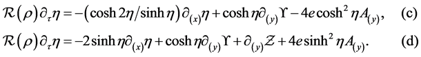 (6.1)
(6.1)
On one hand, according to constraint (2), the r.h.s. of these equations do not depend on radial . On the other hand, according to constraint (1), we have
  in the l.h.s. This is possible only when
  and, as a consequence, when
 . Moreover, the entire r.h.s. of Eqs. (6.1) does not depend on
 ,
,
 (6.2)
(6.2)
By virtue of (5.7), Eqs. (6.2.c) and (6.2.d) constitute a homogeneous linear system for  and
and  with a nonzero determinant and it has only a trivial solution,
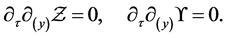 (6.3)
(6.3)
The functions  and
and  cannot depend on
 . Next, consider Eqs. (5.4.b) and (5.4.a), trading there
  for
for  and
and , and differentiate them over
 . Since the fields
  and
and  are static, we have
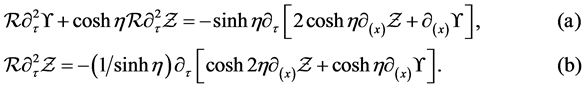 (6.4)
(6.4)
On one hand, nothing in the r.h.s. of Eq. (6.4.b) depends on . On the other hand,
  in the l.h.s. depends only on
 . Thus, the only option is
 , and the second term in the l.h.s. of Eq. (6.4.a) is zero. By the same token,
  , so that
 (6.5)
(6.5)
Next, the r.h.s. of Eqs. (6.4.a) and (6.4.b) yield a homogeneous linear system for  and
and  with a nonzero determinant that has only trivial solution,
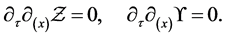 (6.6)
(6.6)
Since , the derivatives
  and
and  in the r.h.s. of (6.4) can depend neither on
  nor on
  and
and . Then, it follows from Eqs. (6.3) and (6.6) that
 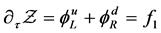 and
and  must be constants. But for a solitary waveform to have constant energy, all its components must oscillate synchronously with its world time
 . These observations can be summarized as
  and
and , which reassures one that the state
  is τ-stationary. The tangent components of tetrad vectors
  and
and  become equal,
  and
and . The tetrad bases
 , (3.9) and
 , (3.16), which are defined over the principal manifold
 , become identical in their
turn. As long as , by virtue of Eqs. (6.1), we must have
 ,
,  , and the t-static
  of the
  -mode must be zero,
 . There remain only two essential parameters,
  of the transformation (3.10), and
  of (3.19). The system (5.4) simplifies to
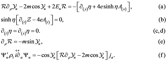 (6.7)
(6.7)
Let us contract Eq. (6.7.f) with , i.e. project it onto the tetrad vector
 . Then
  and
and . Since
  and also
  , the l.h.s. of this equation becomes
 . Hence, the system of equations that defines the shape function
  of the wave form
  reads as
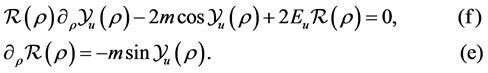 (6.8)
(6.8)
These two equations depend exclusively on radial variable  (or its substitute
 ), and they do not depend on the external field
 . The l.h.s. of Eqs. (6.7.a) and (6.8.f) depend only on
 , so that (6.7.a) naturally splits into (6.8.f) and the difference between Eqs. (6.7.a) and (6.8.f). Since
  , Eq. (6.7.b) can be written down as Eq. (6.9.b) below
 (6.9)
(6.9)
These are the only equations for the mode  depending on external field
 . The result
  follows from the equations of motion, and it leads to yet another constraint that must be imposed on the external field,
 . Substituting here
 , and
, and  from Eqs. (3.21), we arrive at
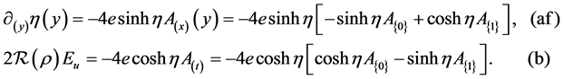 (6.10)
With known external  and
and , Eq. (6.10.af) can be integrated explicitly, and determine the yet unknown function
 . Together with the solution
  of the system (6.8), they determine the permissible component
  of the vector potential, which is compatible with a stable solitary waveform
 ,
,

6.2.  -Mode,
 . The Analysis of Equations
The inward polarized two-component solitary waveform  was conjectured [2] to be unstable it terms of the world time
  (since there was no any other choice). The situation with the four-component
  is more intricate. Insta- bility due to nonlinear effect of the local time speed-up in the interior of an initially localized waveform can be visualized only as a convection current in its exterior, where the energy is defined with respect to time
 ,
, 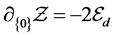 , which is defined by Eqs. (3.19); it was tentatively interpreted as the time coordinate of the tetrad basis
  (see Section 7).
Here, we start with rewriting Eqs. (5.6.c) and (5.6.d) as
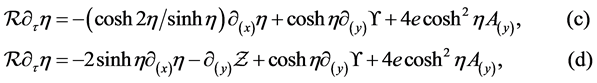 (6.11)
and obtaining, as in the previous case,  ,
,  , and
, and
 (6.12)
which readily duplicates Eqs. (6.2) and (6.3), viz.,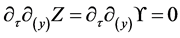 ―this time, for the
  mode. Next, we consider Eqs. (5.6.a) and (5.6.b), trading there
  for
for  and
and , and differentiate them over
 . Since the fields
  and
and  are static, we have
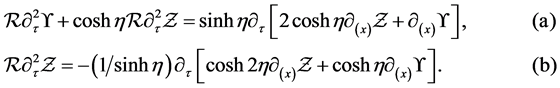 (6.13)
Duplicating the foregoing analysis and presuming that the form  is stable, we arrive at the same Eqs. (6.5), (6.6), and conclude that
  and
and .
.
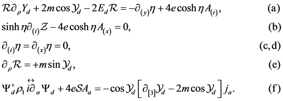 (6.14)
Here,  , and the physical meaning of the constant
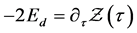 , as well as conditions under which
  can be stable, is yet to be established. As previously, by virtue of Eq. (5.6.d), the t-static
  of the
  -mode must be
zero, 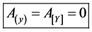 , and
, and . Let us take
  and
and
contract Eq. (6.14.f) with . Then
  and also
 ,
, . Then the l.h.s. of Eq. (6.14.f) becomes
 . After cancellation of the common factor
 , the system of equations that defines the shape
  of the wave form
  reads as
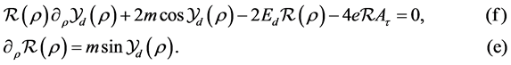 (6.15)
From here, we conclude that ; this component can only depend on radial variable
 . Since
 , the difference be- tween Eqs. (6.14.a) and (6.14.f) and Eq. (6.14.b) can be cast as
 (6.16)
Next, we can rewrite the original  from the r.h.s. of Eq. (6.14.a) as
 , thus separating the scalar potential
  of the electric field and the vector potential
  of the magnetic field. Then, recalling that
  and rewriting Eq. (6.14.b) as
  , one can find that
  and substitute it into Eq. (6.14.a)),
 (6.17)
Clearly, in this equation the radial variable  and the distance y in “alti- tude” angular direction, are not separated. However, the only possibility allowed by this equation is
 , i.e.,
 . Finally, taking the difference between Eqs. (6.17) and (6.15.f) (which is remarkably independent of
 !), we can write it and Eq. (6.14.b) as
 (6.18)
These equations are mutually consistent only when  and, consequently, when
 , which leads us back to the two-component
  -mode, studied in Ref. [2] . A solitary localized solution
 , which was tentatively associated with a negatively charged Dirac particle, does not satisfy the stationary nonlinear Dirac equation with a definite energy. Ergo, the formally obtained solution
  cannot be considered a stable mode at least in the sense that it does not deter- mine the same world time
  over the entire waveform.
6.3. Analytic Solutions in Principal Physical Manifold M
In order to fix a reference point for a further discussion, we begin with reviewing the exact formal solutions of some of the above equations and disregarding for a while further constraints that may invalidate them as physical solutions.
Modulo the notation, the systems of Eqs. (6.8) and (6.15) for the four- component modes  and
and  are the same as were solved in Ref. [2] for the two-component modes
  and
and . Here, we do it differently. Using the nota- tion (3.2), in terms of which
  and
and , we rewrite these systems as
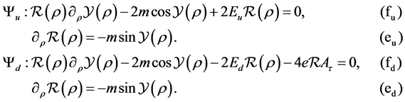 (6.19)
In this form, the equations only differ in the sign of energy. Let  for
for  and
and  for
for .
.
1) Solutions in the absence of external field
When , the two modes share the same characteristic equation,
 (6.20)
Its general solution, depending on one, yet undetermined constant C, is
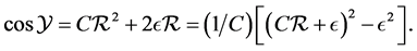 (6.21)
Then, Eqs. (6.19.f) are reduced to the following equivalent forms:
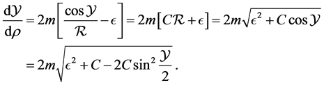 (6.22)
The last one of these forms is immediately connected to the incomplete elliptic integral of the first kind12. For  determined by Eq. (2.22) to be aperiodic function, it is n.a.s. that
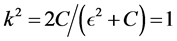 , i.e., that
 . Then,
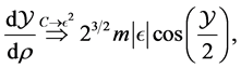
and integration of this equation becomes elementary,
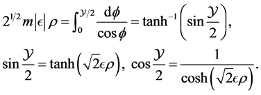 (6.23)
The sign of  remains the only yet undetermined parameter. Obviously,
  , and
, and . Next, we readily have
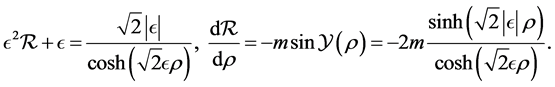 (6.24)
When , we have
 , which is possible only when
 . Therefore,
  while
while . For an on-mass-shell solution with
  (and thus, with
 ) the “vacuum level”
  emerges as the consequence of local time slowdown, i.e., of the Dirac equations of motion! The corresponding solutions for
  are as follows:
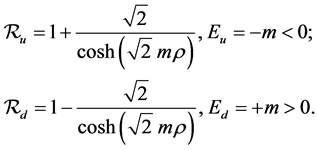 (6.25)
The solution  has a bump of invariant density near the center and a negative energy
 , while
  has a dip and a positive energy
  13. The affine curvature
  reaches its theoretical maximum at the inflection point
 , where
  and
and . The curvature monotonously decreases not only with the increase of the radial parameter at
 , but also with its decrease at
 , which is counterintuitive. A new radial variable
 , introduced in Eq. (3.22) looks like a plausible solution for this discrepancy, which contaminates both modes. When
 , we also have
  . Consequently, at large distances,
  and the proper time within the mode
  flows slower/ faster than the world time
  as if there was an attractive/repulsive “Newton’s potential”
 , i.e.,
  (without any allusion to gravity!).
Finally, for the mode , the invariant density reaches its theoretical minimum at
 ,
, . At
. At , the density
 , as formally defined by (6.25), becomes negative, which is impossible. This can be a yet another indication that an isolated localized negative charge is unstable (cf. Eq. (6.18.a) and the following comments). Furthermore, when
  (or
(or ,
, ), the spacelike vectors
  and
and  of the tetrad (3.9) become null vectors, and only the directions of
  and
and  become lightlike. The entire picture looks like a propagating discontinuity along a characteristic of a hyperbolic system. Such pattern just cannot belong to a stable configuration. The enigmatic void at the center of the mode
  (an electron), if properly under- stood, leaves space for a much smaller positive charge (a proton) with
 , which is another body that need not share the same “world time”
  with the electron even in the ground 1s-state of the hydrogen atom.
An important observation must be made regarding the sign of electric charge. The invariant density  is the sole component
  of the vector current in the basis
 . It is associated with the charge density and, as it is well-known for the classical Dirac field, it is strictly positive, while the energy can have both signs. In QED this apparent problem is resolved through the postulate of the Fermi-quantization. At the same time, on every reasonable account, the electric charge density is the divergence of its electric field. Obviously, uniform charge distribution does not produce any electric field. Therefore, if we subtract from the invariant density (6.25) the uniform “vacuum part = 1”, then the remainders,
  and
and , will have opposite signs, which then can be associated with the sign of a charge. Together with well- motivated autolocalization, this picture seems to be a classical equivalent of the so-called Dirac sea, which avoids the enigmatic concept of the completely occu- pied states of negative energy.
2) Solutions in external coulomb field
Because of the stringent constraint (6.18),  , only the two-component
  can be stable as a solitary autolocalized waveform and admit an external centered Coulomb field. Obviously, the latter can be defined only in the ambient
  as
as , and then mapped onto
  as in Eq. (3.20), viz.
 . Thus, the system (6.15), which determines the shape of wave- form, becomes
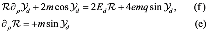 (6.26)
Introducing the phase shift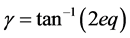 , we can rewrite Eq. (6.26) as
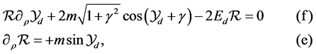 (6.27)
so that the effect of the Coulomb field is encoded into the phase shift . Even characteristic equation of this system,
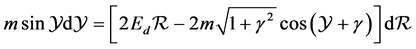 ,
,
is an extremely complicated difference-differential equation [12] . Though it is tempting to view it as a candidate for the description of a hydrogen atom within framework of MIAG, the problem of solving this equation is beyond the scope of this paper. It is very likely that stable solution without the lightlike singular surface at  is possible only with Coulomb electromagnetic potential, which could have been an unusual way to derive Maxwell equations. By all means, this is not a one-body problem.
7. Autolocalized Dirac Waveforms in R4: View from the Outside
In Section 6 we analyzed and solved the equations for Dirac currents of Section 5, using the time variable , which is defined on the physical manifold
 . Here, we reconsider this analysis from the viewpoint of the ambient
 , where the points are normally associated with events. As long as a solitary waveform can participate an event only as a whole, it is virtually impossible to resolve its internal structure while preserving a stable configuration. The immediate goal of this section is to demonstrate that ignoring the local time slowdown almost wipes out the effect of autolocalization. It also makes impossible to have stable waveforms of a constant energy with respect to the time
  of external observer.
7.1. Analysis of the Reduced Equations in R4
As previously, we begin with the system (5.4) for the mode  and with (5.6) for the mode
 . As it has been discussed in Section 3.3, we will be able to use angles
  instead of the angular arcs
 ,
,
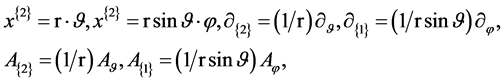 (7.1)
(7.1)
where  is the radial distance compatible with the affine curvature,
 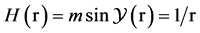 (as in Eqs. (3.22) and (3.23)). Since
  , and all transformations of the tetrads, from
  to
to , are the Lorenz boosts in
 , the new analysis is not much different from the previous one. The new time variable will be the anholonomic world time of an inertial rest frame of an external observer with the grid of clocks synchronized by signals, and not the locally defined world time
 . Hence, an important segment of nonlinear dynamics will be lost. The field theory, practically and in its spirit, is strictly local, which is especially true when equations of motion are nonlinear. In this respect, the MIAG resembles the general relativity, where the clocks also cannot be synchronized and attraction of the material bodies is due to the local time slowdown.
1) The  -mode,
 . Using Eqs. (3.21) to rewrite, in all equations of the system (5.4), the directional derivatives and components of the vector potentials with respect to the tetrad
 , we obtain
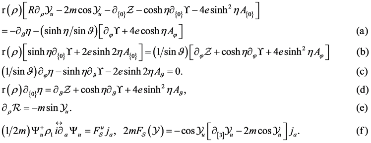 (7.2)
(7.2)
Since , we also have, by virtue of Eq. (c),
 . Since
 ,
,  and
and  in the r.h.s. of Eq. (d) do not depend on
 , then
 . Modulo the notation, next step reproduces Eqs. (6.2) and (6.3) with the conclusion that
 , so that the functions
  and
and  cannot depend on
  and, by virtue of Eq. (d),
 . Next, consider Eqs. (7.2.b) and (7.2.a) and differentiate them over
 . Assuming, as previously, that the fields
  and
and  are static, we have, instead of (6.4),
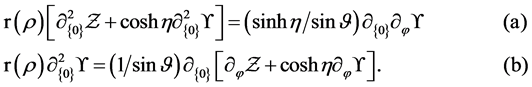 (7.3)
(7.3)
Since the r.h.s. of both equations do not depend on , we have
  and then,
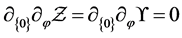 . Hence,
  and
and  can be only constants, while
  and
and  cannot depend od
 . The same considerations as before prompt the conclusion that
  and
and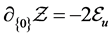 . Then Eq. (b) yields,
  and the system (7.2.a,e) is reduced to
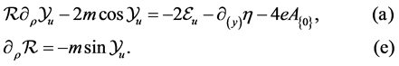 (7.4)
(7.4)
Obviously, this system is not compatible with the Eq. (7.2.f), which does not depend on .
.
2) The  -mode,
 . Similar analysis of the system (5.4) (which the reader can easily reproduce) ends up with equations
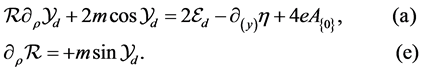 (7.5)
(7.5)
which differ from (7.4) only in signs of  and
and .
.
7.2. Analytic Solutions in Coordinate Manifold R4
Notably, unlike in Eqs. (6.19), Eqs. (7.4.a) and (7.5.a) both depend on the external field  and the energies
  are not accompanied by the factor
 . The latter originated from the slowdown of the local time
 , which is the genuine intrinsic mechanism behind autolocalization. Here, we start with Eqs. (7.4) and (7.5) that were derived using the time variable
  associated with an external observer and consider the case when
  and
and . We choose to follow the phase difference
 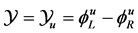 and, by virtue of (3.2),
 .
.
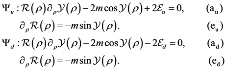 (7.6)
(7.6)
The characteristic equation of the system (7.6) and its solution are as follows
 (7.7)
(7.7)
where, as previously,  for
for  and
and  for
for . Now, Eqs. (7.6.a) become as follows,
 (7.8)
(7.8)
where the expression under the square root must be positive. There are two cases when the function , determined by Eq. (7.8), is aperiodic function of radial variable
 . Namely, when
  and
and , then
This is the standard case when , and an elementary inte- gration yields,
 (7.9)
(7.9)
When , the integral diverges at the upper limit, so that, as one would expect,
  and the four-component
  becomes the two-component
  when
when . When
 , then
  and, by virtue of (7.7), the “vacuum level” is
 . This result still is the conse- quence of equations of motion, but the complete set of constraints, which could have guarantee the stability, is not satisfied. Furthermore, in this vacuum, all Dirac currents become lightlike (or null-) vectors, which is possible only on the singular two-dimensional surfaces. Since the constant C remains undetermined, these solutions cannot be considered autolocalized. As it was previously in
 , the energies of two modes have opposite signs,
  and
and . Another aperiodic solution could have corresponded to
 , and
, and . However, it is the same solution (7.9) (cf. footnote12).
Since now Eq. (7.7) is reduced to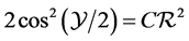 , the distribution of invariant density becomes as follows,
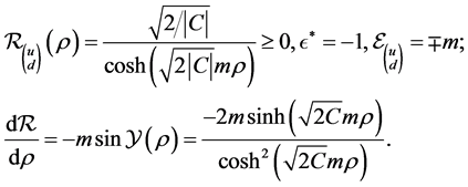 (7.10)
Both  and
and  have a magnified invariant density with respect to vacuum level zero. In these equations, the constant C is still a free parameter, which is not consistent with autolocalization. This is in contrast with Eqs. (6.25), where the intrinsic nonlinearity of the Dirac equation had left no freedom of normalization. In terms of the time
  of an external observer, there is no local time slowdown, which is the main nonlinear physical effect behind autolocalization in
 . The inhomogeneous distribution of the invariant density is due to a much weaker effect of the non-vanishing pseudoscalar density. As a consequence, in order to get charges of both signs, one must resort to Fermi-quantization along with an enigmatic concept of the “Dirac sea” of com- pletely occupied states of negative energy.
8. Summary and Outlook
Here, we are going to review the results of this two previous papers [1] [2] and outline several unsolved problems. Although we keep in mind the understanding of the origin of charge asymmetry of observed matter as the final goal, this asymmetry is inseparable from the problem of field localization into finite sized objects. The proper time slowdown as the generic mechanism of autolocalization, was proposed in Ref. [1] along with a novel kind of matter-induced affine geometry. The existence of two major types of localized solutions (stable and unstable) of the nonlinear Dirac equation was demonstrated in Ref. [2] .
The Lorentz-like mathematical structure of MIAG is solely due to the algebraic properties of the Dirac field, and it clearly discerns the inward and outward directions within a waveform. But, once a localized form is stable, it can respond to any conceivable measurement only as a whole. Within a stable solitary waveform there can be neither events nor test particles, signals, clocks and rods (which makes it very different from another nonlinear theory, the general relativity). The geometry of its interior can only be affine. In order to learn if the Dirac field can determine a metric, one has to solve at least a two- body problem.
An important result discovered within MIAG is that the a priori expected perfect dynamical spherical symmetry of  appears to be broken down to the axial symmetry of the solution, which is consistent with the anticipated internal polarization of a Dirac particle. Indeed, the first one of the transformations (3.16),
  , is akin to the gauge transformation (cf. [1] , Eq. (4.5)). The second one,
  , is the transition to a rotating system of the intermediate tetrad
 . The last transformation (3.19) is between
  and the tetrad
  of the preferred coordinate system
 . The polar axis of the stationary waveform is fixed by the Dirac currents in
 , but it is totally arbitrary in
 . Neither uniformity nor isotropy of ambient space is broken by the presence of a solitary waveform, which guarantees that its total linear and angular momenta are conserved.
Among all quantities of dynamic origin that MIAG is dealing with, only one can be associated with a length, viz., the curvature of affine sphere with constant radial parameter ,
,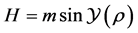 . Since
 ,
,  cannot be considered a distance. In fact, according to Eq. (6.24),
 ;
;
this function monotonically increases, in compliance with our intuition, from zero at  to its maximal value
  at the inflection point
  of the curve
 . But then, defying our three-dimensional intuition, it mysteriously drops to zero at
 . If not this abnormality, the formal mismatch between affine curvature
  and radius
  could have been easily eliminated by choosing such a new radial variable
 , Eq. (3.22), that
 . This could have been the first step towards a metric geometry, if we had
 . Unfortunately,
 ; the variable
  does not cover the domain
 . The inverse function
 , given by Eq. (3.23) is double-valued. The “exterior” (
 ) and “interior” (
 ) of the waveform correspond to different branches of this function. Yet, an open question is if the boundary
  (or
(or ) is physical, or is it an artifact of poorly chosen variable
 . The answer clearly depends on the type of a waveform, which determines the function
 .
.
For stable solitary “positron” or “proton”, as is well known, an attempt to resolve its structure at the distances below Compton wavelength  causes creation of additional particles. This may correspond to such external fields (e.g., of gamma-photons) for which differential identities (6.10) do not hold, and the
  -configuration becomes unstable. Once again, this is not a one-body problem. For a stable proton, the branch
  of the function (3.23) must be considered unobservable, though the space inside radius
 , where
 , is not “empty”.
For the unstable solitary “electron”, the situation is totally different. The invariant density of the  -mode reaches its theoretical minimum,
  , at
, at . When
 , the density
 , as formally defined by (6.25) in the absence of external field, becomes negative, which is impossible. Here, the branch
  of function (3.23) is just absent. One may think of the domain
  as an “empty space” where
  and all Dirac currents are either null or lightlike. But such a domain can only be a singular two-dimensional surface. The most natural conjecture is that it is incorrect to rely on Eq. (6.19.fd) without the external field
 . The Coulomb field of a proton placed in empty interior of an electron will considerably modify the function
 , but the Coulomb field will not be electrostatic in term of the world time
  of the electron. Mathematically, the shape of
  -waveform will be governed by Eqs. (6.27), which cannot have so simple solutions as (6.25), just because these are the differential-difference equations [12] . Physically, the ratio of proton and Bohr orbit radii is about
 , so that the nonlinearities, which are effective only at distances of the order
 , will be negligible.
In the course of this study, we have explored two different approaches to the stability of autolocalized waveforms. The simplest one, which was used in Ref. [2] for the two-component solutions, alludes to the perturbation theory and is readily reproduced for the case of four-components. Indeed, let us assume that in Eqs. (B.6) and (B.7) for the “stable” mode  we have
 , which means that
  (because
 ). Next, multiply Eq. (B.6) by
  and (B.7) by
  from the left, thus converting them into equations for the “matrix elements”. There is only one term in Eq. (B.7), that can be responsible for conversion of large initial
  to small final
 , namely
  . It stems from the ladder operator
  which flips
  in the Dirac equation (2.5). However, this term is suppressed by a small factor
 . Conversely, in Eqs. (B.13) and (B.14) for the “unstable” mode
  we have
 , which also means that
  (because
 ). The term, which can cause conversion of large initial
  to small final
  in Eq. (B.13) is
 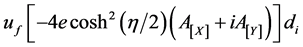 ; it comes from the ladder operator
 , that flips
  in the Dirac equation (2.5)14. Here, the factor
  and this transition is not suppressed, which hints instability of the
  -mode. This simplistic analysis, which views instability as a process, conflicts with the spirit of MIAG that aims at finding the cosmologically stable states. In order to deal with the transient processes, we still have to learn how to deal with two bodies, propagating waveforms, etc.
A more thorough approach is taken in this paper. To be precise, in scope of MIAG, the equations of motion are being solved not for the Dirac field , but for the four so-called Dirac currents, which are more closely connected with the observables. Equations that govern their dynamics are the differential identities derivable from the original Dirac’s system of PDE. They do not just replace the equations of motion. They also serve as a set of consistency conditions, which are needed to filter out the stationary/stable autolocalized solutions. Those waveforms that do not satisfy all of them, are not considered the solutions.
All differential identities appear to be satisfied for the outward polarized  -mode (with the axial current looking outward and a magnified invariant density
  at the origin). At most, some of them impose relatively weak restrictions on the external field
 , without affecting shape of the waveform
 . This mode is stable. For the inward polarized
  -mode (with the axial current looking inward and a reduced invariant density
  at the origin), two identities, each of which could have determined the shape of a solitary waveform, are conflicting. This mode cannot be stable.
There also are other intriguing physical questions.
1) As it was pointed out long ago by A.Eddington [13] in connection with the bound state problem, “a proton today and an electron yesterday do not consti- tute a hydrogen atom”. From perspective of MIAG, the same problem sounds as follows. Being considered as autolocalized waveforms, do electron and proton determine a common world time  across the hydrogen atom? Obviously, the answer is negative because electron and proton are two different waveforms and it is unlikely that Dirac theory of hydrogen atom can be reduced to three spatial dimensions.
2) So far, the static fields  and/or
  in constraints like (6.10) and (6.16) were considered the external fields. Should/can they also have the Dirac field of the waveform as their source. Whatever the answer will be, it will clarify if Maxwell equations are the constraints required by the Dirac equations.
3) Is there a way to determine orientation of the aforementioned preferred coordinate system when there is no external fields? In other words, is solitary proton similar to a magnetized needle?15 The reader can view the last question as a version of the Mach paradox.
4) Finally, the biggest challenge is to find a regular method to treat the transient processes with the Dirac waveforms in order to study how auto- localization may develop in time. Now we know that the internal spherical symmetry of a stable waveform is broken to the axial one. Therefore, we can read the chain of transformations (3.16) in the opposite direction, starting with the preferred tetrad,  , i.e.,

Can the ubiquitous magnetic field lower the threshold amplitude of fluctua- tions, after which the local time slowdown takes over the dynamic of fluctua- tions? Does the magnitude of magnetic field matter? If so, it is reasonable to look, for example, for a correlation between the observed excess of positrons in cosmic rays and strength of magnetic fields in their potential sources (for a recent review see Ref. [15] ).
Acknowledgements
I am indebted M.E. Osinovsky for his advice on subtle issues of differential geometry and for critically reading the manuscript. This work is supported by the Rapid Research, Inc.
Cite this paper
Makhlin, A. (2017) On the Origin of Charge-Asymmetric Matter. III. Properties of Autolocalized Dirac Waveforms. Journal of Modern Physics, 8, 1478-1519. https://doi.org/10.4236/jmp.2017.88090
References
- 1. Makhlin, A. (2016) Journal of Modern Physics, 7, 587-610
https://doi.org/10.4236/jmp.2016.77061 - 2. Makhlin, A. (2016) Journal of Modern Physics, 7, 662-679
https://doi.org/10.4236/jmp.2016.77066 - 3. Sakharov, A.D. (1967) JETP Letters, 5, 24-27.
- 4. Takabayasi, T. (1958) Nuovo Cimento, 7, 118.
https://doi.org/10.1007/BF02746891 - 5. Takahashi, Y. (1983) Journal of Mathematical Physics, 24, 1783.
https://doi.org/10.1063/1.525896 - 6. Levi-Civita, T. (1926) The Absolute Differential Calculus. Blackie & Son Limited, London. (Dover, 1977)
- 7. Tamm, I. (1930) Zeitschrift für Physik, 62, 545.
- 8. O’Neill, B. (1966) Elementary Differential Geometry. Academic Press, New York.
- 9. Stoker, J.J. (1969) Differential Geometry. Wiley Interscience, New York, London, Sydney, Toronto.
- 10. Makhlin, A. (2010) Localization, CP-Symmetry and Neutrino Signals of Dirac Matter, arxiv:1005.2693[math-ph].
- 11. Byrd, P.F. and Friedman, M.D. (1971) Handbook of Elliptic Integrals for Engineers and Scientists. 2nd Edition, Springer-Verlag, New York, Heidelberg, Berlin.
https://doi.org/10.1007/978-3-642-65138-0 - 12. Bellman, R. and Cooke, K.L. (1963) Differential-Difference Equations. Academic Press, New York & London.
- 13. Eddington, A. (1936) Relativity Theory of Protons and Electrons. University Press, Cambridge, p. 110.
- 14. Schwinger, J. (1973) Particles, Sources, and Fields. Addison-Wesley, Reading, MA.
- 15. Kruskal, M., Ahlen, S.P. and Tarlé, G. (2016) The Astrophysical Journal, 818, 70.
https://doi.org/10.3847/0004-637X/818/1/70
Appendix
A. Notation and algebraic conventions
All observables associated with the Dirac field are bilinear forms built with the aid of Hermitian Dirac matrices  and
and , which satisfy the commutation relations
 (A.1)
(A.1)
Throughout this paper, the Dirac matrices  associated with a tetrad
  are numeric and are chosen in the spinor representation,
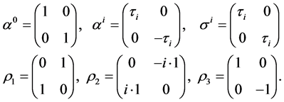 (A.2)
(A.2)
where  are the
  Pauli matrices. The Dirac matrices,
  (
( ,
, ,
, ), and
  satisfy the same commutation relations as the Pauli matrices, and all
  matrices commute with the
  matrices:
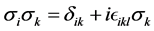 ,
, 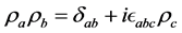 ,
,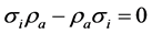 . The matri- ces
  and
and  are commonly known as
  and
and , respectively16.
If the Dirac spinor is written down in terms of modules and phases of its components,
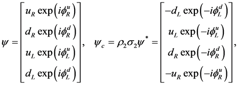 (A.3)
(A.3)

16We consciously refrain from using the anti-hermitian matrices  and the Pauli-conju- gated spinors
 . In their terms, the formulas of parallel transport would be much less transparent and unnecessarily complicated.
then, with the Dirac matrices (A.2), the scalars and the four Dirac currents have the following components,
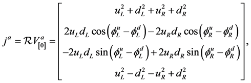
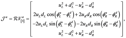 (A.4)
(A.4)
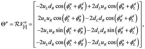
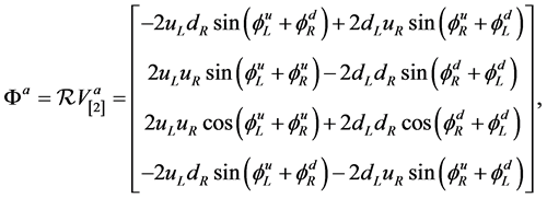 (A.5)
(A.5)
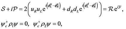 (A.6)
(A.6)
 (A.7)
(A.7)
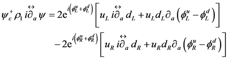 (A.8)
(A.8)
B. Transformation of the Dirac system (3.5)
The differential operators  are assembled in Eq. (3.5) in the combina- tions, listed below. Denote
  as a shorthand notation for the operator
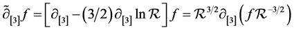 . As in Eq. (3.17), we denote,
  and
and . In what follows,
  and
and 
are the notation that must be expanded according to (3.14), viz., 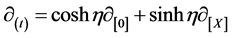 and
and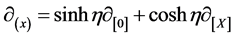 .
.
1. The  mode. When the axial current is directed outward (or up;
 ), then the operators in the Dirac equation (3.5) are,
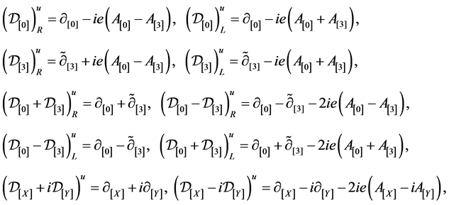 (B.1)
(B.1)
where, in line with notation (A.3), the subscripts R and L discern between action on right and left components, respectively. The first and the third equations of the system (3.5), which are multiplied by  and
and , respectively, read as
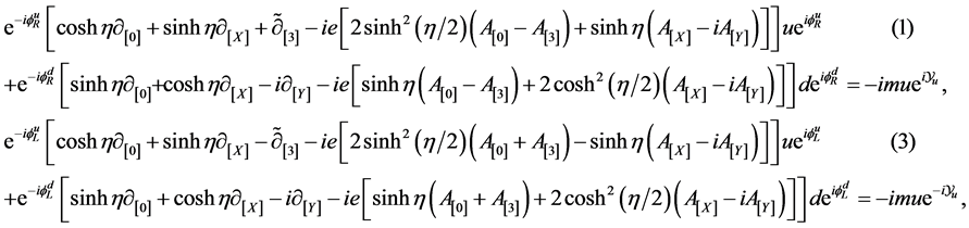 (B.2)
(B.2)
where  and
and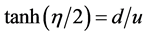 . In the l.h.s. of equations of the system (3.5) it is fairly simple to split derivatives of amplitudes and phases. Indeed, we have,
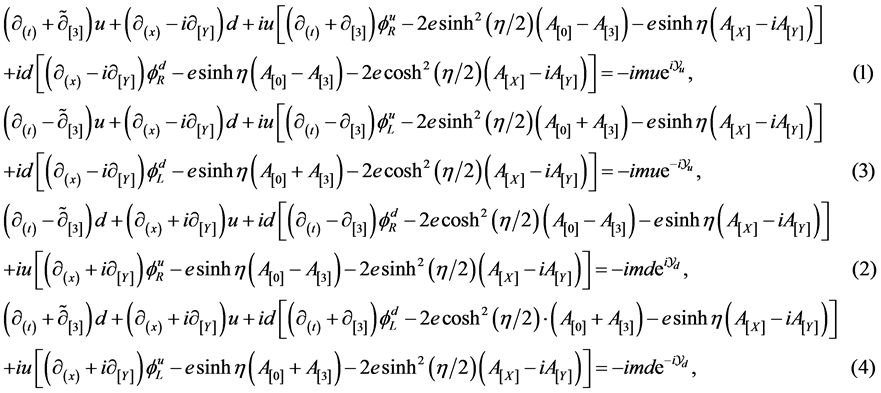 (B.3)
(B.3)
The differences between Eqs. (B.3.1) and (B.3.3) and between Eqs. (B.3.2) and (B.3.4) can be cast as
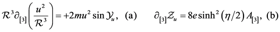 (B.4)
(B.4)
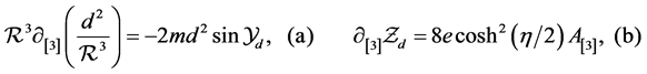 (B.5)
(B.5)
for real (a) and imaginary (b) parts, respectively. In imaginary part we took into account that due to Eqs. (3.4), ;
;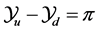 . Next, take sums of Eqs. (B.31), (B.3.3) and of Eqs. (B.3.2), (B.3.4) and proceed in the same way,
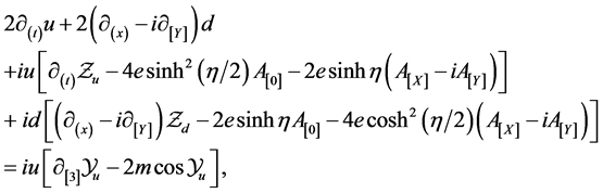 (B.6)
(B.6)
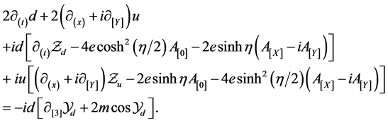 (B.7)
(B.7)
2. The  mode. For the axial current directed inward (or down;
 ), we have
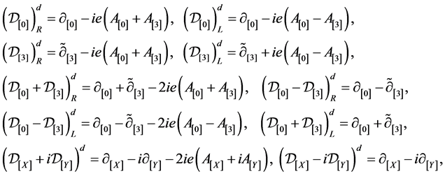 (B.8)
(B.8)
which is different from (B.1) due to the pointed out earlier interplay between signs of  and of
 . Now, the second and the fourth equations of the system (35) read as
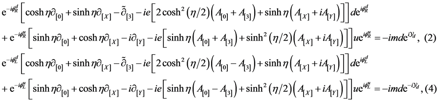 (B.9)
(B.9)
Here, since ,
,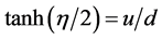 . In the l.h.s. of these equations, we split derivatives of amplitudes and phases. Then we have,
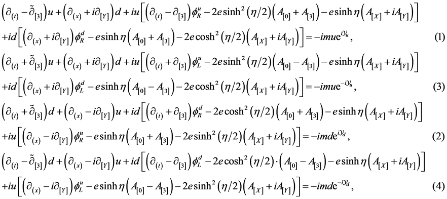 (B.10)
The differences between Eqs. (B.10.1), (B.10.3) and between Eqs. (B.10.2), (B.10.4) can be cast as
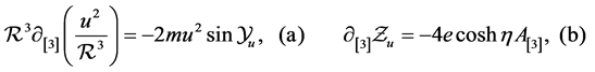 (B.11)
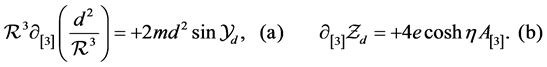 (B.12)
which replace Eqs. (B.4) and (B.5).
Next, take sums of Eqs. (B.10.1), (B.10.3) and of Eqs. (B.10.2), (B.10.4) and proceed in the same way. The result replaces Eqs. (B.6) and (B.7),
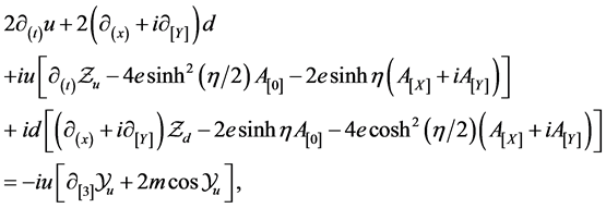 (B.13)
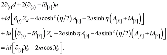 (B.14)

Submit or recommend next manuscript to SCIRP and we will provide best service for you:
Accepting pre-submission inquiries through Email, Facebook, LinkedIn, Twitter, etc.
A wide selection of journals (inclusive of 9 subjects, more than 200 journals)
Providing 24-hour high-quality service
User-friendly online submission system
Fair and swift peer-review system
Efficient typesetting and proofreading procedure
Display of the result of downloads and visits, as well as the number of cited articles
Maximum dissemination of your research work
Submit your manuscript at: http://papersubmission.scirp.org/
Or contact jmp@scirp.org
NOTES
1Since it is impossible to place rods and clocks within a stable solitary waveform, the proper time  is defined as a parameter along the lines of the timelike vector current (as if they were trajectories of the test-particles). The world time
 , which is the same over entire waveform, enumerates the normal hypersurfaces, which are orthogonal to the congruence of lines of the vector current. The main result of the MIAG is that
 , where the sign of
  coincides with the sign of the charge.
2All notation and definitions are the same as in Refs. [1] , [2] ; see Appendix A. We use the system of units where  and, accordingly,
  ,
, . To avoid any ambiguity, especially when indices that numerate tetrads take special values, the latter are written down in brackets, parenthesis, or braces. The indices
  numerating the original tetrad of the Dirac currents,
  , are written down in brackets. The numbers or letters that stand for indices
 , which numerate the tetrad vectors
  are written down in parentheses. Bold kernel letters assume an omitted coordinate index
 , which belongs to the ambient coordinate space
 . The tetrad indices of the
  are enclosed in braces, e.g.,
 .
.
3In context of differential geometry, it is always possible to choose a principal n-th congruence and then augment it (in general, in more than one way) with n − 1 conjugated congruences, forming a canonical system of mutually orthogonal congruences [6] . In our case, the radial congruence is the principal one due to equations of motion and is physically motivated by autolocalization, while the canonical system is always given by a set of the Dirac currents.
4Having no metric, we assume here geodesic of an affine space, i.e. such a line  that its tangent vector,
 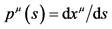 , is parallel-transported (with respect to an affine connection
 ) along the line,
 . In our particular case of the tetrad vector
 , this amounts to
5It is worth reminding, that tetrad , which has been formally introduced in Ref. [1] , is a quadruple of linearly independent vectors
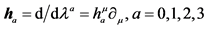 , (with the non-degenerate matrix
 ,
, ). Then there also exists the inverse matrix
  of the 1-forms
  so that
  and
and . Obviously, the formally introduced objects,
 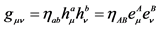 and
and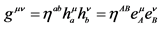 , can be used to move the coordinate (Greek) indices up and down. With
  thus defined, we also have the formal relations
  and
and , which can be interpreted as orthonormality relations for the tetrad bases
  and
and  if we postulate that this
  determines a fundamental tensor in coordinate basis. However, in general, this is not the metric that governs propagation of signals at a larger scale.
6It will be found later, that equations for stationary solitary waveforms allow only for the value .
.
7Looking forward to the future study of the transient processes, one must keep in mind, that  is an harmonic function and that
  is defined up to an additive harmonic function. Therefore, both
  and
and  (or their derivatives of some order) can have discontinuities along characteristics of the wave equations,
  and
and . The leading fronts of all signals (including those of the Dirac field) propagate along characteristics.
8The presence of the vectors  and
and  in the tetrad is necessary not only from geometric perspective (without them the tetrad would be incomplete). In fact, they are the matrix elements of transitions between the Dirac field and its charge conjugate (between the states of the positive and negative energy). The existence of transitions into intermediate charge-conjugated states and accompanied by the spin-flip, is vital even for basic QED processes like Compton scattering, which is a well- known fact. It is rarely emphasized, that namely these transitions, alone, completely determine the classical long-wave limit of the Compton process (Thompson scattering) [7] . In modern language, the pole of the propagator of the positive-energy intermediate states in Compton process is strictly fixed by the total energy (because this is the s-channel), and it does not contribute to the angular distribution of the scattered photons. All angular dependence comes from the propagator of the negative-energy intermediate states (which is similar to the propagator of the t-channel potential scattering and thus accounts for all partial waves). In the context of the transient processes, it is also possible to trace a deep physical connection between this property of the Compton scattering and the classical Ewald-Oseen’s extinction theorem.
9All points of an umbilical manifold are umbilical. A point P is called umbilical if all principal curvatures at this point are equal, so that all tangent directions at a point P are equivalent. Spherical symmetry of solitary waveforms is very intuitive and is usually taken for granted. But it appears that Dirac field respects our intuition that was developed back in the classical physics. The Dirac equation becomes nonlinear and yields solitary autolocalized solutions, which stunningly resemble, by their properties, natural objects. A proof that spherical ansatz (3.1) is the only possible option would be a paraphrase of the well-known Birkhoff theorem that any spherically symmetric solution of the vacuum field equations must be static and asymptotically flat. This means that the spacetime outside of a spherical, non-rotating, gravitating body must be given by the Schwarzschild metric. The condition (3.20) singles out the Schwarzschild coordinates among many possible ones.
10Technically, it is necessary to substitute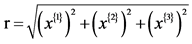 ,
, 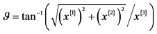 and
and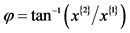 .
.
11This result is more general that it may seem, because one can safely impose the gauge condition . The corresponding gauge transformation is well defined, viz., let
  be an arbitrary field configuration and
  its gauge transform with the generator
  , then the new field,
  , obeys the condition
 . Importantly,
  is a holonomic coordinate so that the path ordering
  is unambiguous.
12 ,
, . Its inverse is a well- known Jacobi’s amplitude function,
 . The Jacobi’s elliptic functions
 ,
,  and
and  are known to be double-periodic functions of their argument. When
 , the periodicity disappears (the period becomes infinite and the integrals
  become elementary (hyperbolic) aperiodic functions [2] , [11] .
13The second aperiodic solution would correspond to . Then
 , and the indefinite integral,
  , is infinite at
  and zero at
 . This is the same solution (6.19)-(6.25) but with
 , viz.,
  and
and .
.
14With all phases recovered, this matrix element is as follows,  (the same holds for the
 ) [2] . This matrix element, as expected, oscillates as
 , which can be viewed as a precursor of Schrödinger’s Zitterbewegung.
15As J. Schwinger pointed out in Section 4.2 of his book [14] , the anomalous magnetic moment is a dynamic quantity, which is suppressed over very short time intervals. It is not unreasonable to ask if the same can be true for the normal magnetic moment.