Journal of Transportation Technologies, 2012, 2, 50-62
http://dx.doi.org/10.4236/jtts.2012.21006 Published Online January 2012 (http://www.SciRP.org/journal/jtts)
Multi Model Criteria for the Estimation of Road Traffic
Congestion from Traffic Flow Information Based
on Fuzzy Logic
Hari Shankar, P. L. N. Raju, K. Ram Mohan Rao
Geoinformatics Division, Indian Institute of Remote Sensing, Dehradun, India
Received September 26, 2011; revised October 28, 2011; accepted November 20, 2011
ABSTRACT
In this study, the road traffic congestion of Dehradun city is evaluated from traffic flow information using fuzzy tech-
niques. Three different approaches namely Sugeno, Mamdani models which are manually tuned techniques, and an
Adaptive Neuo-Fuzzy Inference System (ANFIS) which an automated model decides the ranges and parameters of the
membership functions using grid partition technique, based on fuzzy logic. The systems are designed to human’s feel-
ings on inputs and output levels. There are three levels of each input namely high, medium and low for input density,
fast, medium and slow for input speed, and five levels of output namely free flow, slow moving, mild congestion, heavy
congestion and serious jam for the road traffic congestion estimation. The results, obtained by fuzzy based techniques
show that the manually tuned Sugeno type technique achieves 72.05% accuracy, Mamdani type technique achieves
83.82% accuracy, and Adaptive Neuro-Fuzzy Inference System technique achieves 88.23% accuracy. ANFIS technique
appears better than the manually tuned fuzzy technique, and also the manually tuned fuzzy technique gives good accu-
racy which leads that the fuzzy inference system can capture the human perception better through manual adjustment of
input/output membership functions.
Keywords: Fuzzy Inference Systems; Fuzzy Rules; Congestion; Human Perception
1. Introduction
In general, the road traffic congestion of urban transport
is defined as the ratio of volume to the capacity of the
road [1,2]. However, the volume and capacity (demand)
of the road are not directly measurable quantities and
thus the value of congestion becomes subjective in nature.
Hence, in this paper the directly and precisely measur-
able quantities such as density and speed of the vehicles,
are used for the estimation of road traffic congestion [3].
These two traffic parameters are considered in this paper
by keeping in mind that general perception about the
congestion on the roads increases when the number of
traffic (traffic density) increases and also increases when
the speed of the traffic decreases. By the same terminol-
ogy the road traffic congestion can be defined as the ratio
of density to the speed of the vehicles. These two pa-
rameters are the inputs to the fuzzy model, and the output
of the model is level of congestion. In fact, the actual
traffic conditions are not perfectly matches with the con-
ventional way of determining the congestion level using
volume and capacity, because there are a number of other
factors which affect the congestion and also depends
upon the human feelings [4]. But using these directly
measurable quantities, the subjectivity of the conven-
tional method of determining congestion level using
volume to capacity ratio is removed.
The road traffic congestion is one of the most confus-
ing tasks, because there is no standard way of measuring
congestion level on the roads and intersections. It results
in serious environmental, time wastage, health hazards,
and economic problems. Thus, it is very important to
detect where the congestion occurs, as well as to measure
and estimate how the congestion is. There may be a
number of solutions of road traffic congestion like road
pricing, fuel levies, expansion and improvisation of rail-
way lines, and elimination of roundabouts. The main
objective of this study is to estimate the road traffic con-
gestion using fuzzy techniques. Therefore, the fuzzy
techniques are used to tackle this problem by using the
traffic flow information such as speed and density of the
vehicles. The fuzzy logic is well known to be suitable for
handling problems that are nonlinear in nature such as
human feelings [5,6]. Road congestion is a subjective
quantity, because it comes from the feelings of vehicle
driver and decision makers which may be different for
different drivers or decision makers. In the same road
C
opyright © 2012 SciRes. JTTs

H. SHANKAR ET AL. 51
conditions, some may feel that the road is heavily con-
gested, while some others may feel that the road is only
slightly congested. This is the problem of mismatching
data interpretation due to different user’s perception. In
traveler navigation system, publication of congestion
degree will provide drivers useful information, thus, re-
duce traffic jam, increase efficiency of trips, and avoid
wastage of fuel consumption. It is well known that the
process from free flow to serious jam is continuous. It
can be represented by a continuous number, say level of
congestion (LOC). The LOC is related to the basic traffic
parameters such as speed and density. There are other
traffic parameters also which affects the congestion level
but in this study we use only two traffic parameters i.e.
speed and density, which affect mostly to congestion.
The objective of this study is to estimate the level of
congestion of a road segment using different fuzzy mod-
els namely Sugeno-type Fuzzy Inference System, Mam-
dani-type Fuzzy Inference System and Adaptive Neuro-
Fuzzy Inference System [7], to evaluate the performance
of fuzzy inference systems by measuring accuracy of
system outputs against human opinion.
2. Study Area
Dehradun city is chosen as the study area for assessing
the traffic congestion. A road segment with two lanes
from Inter State Bus Terminal Dehradun to Saharanpur is
taken as a test case to quantify the road traffic congestion.
Figure 1 shows the study area depicting the road net-
work of Dehradun city. This road segment has two lanes,
going from ISBT Dehradun to Saharanpur, near ISBT
Dehradun Uttarakhand. In this research framework, five
levels of congestion are defined for traffic congestion,
namely free flow, slow moving, mild congestion, heavy
congestion and serious jam, and estimating them by us-
ing only traffic video.
3. Literature Review
Porikli and Li, 2004 determine five level of congestion
from traffic flow information and video images using a
Hidden Markov Model [8]. Atikom and Pongpaibool,
2006 estimates the road traffic congestion by using vehi-
cle velocity [9]. Krause and Altrock, 1996 uses fuzzy
logic to determine six discrete levels of congestion [10].
The system use velocity and vehicle density as inputs its.
fuzzy inference system. Sule, 1988; Jia and Li, 2003 uses
different factors which affect the road traffic congestion
[11,12]. This study also uses fuzzy inference systems, but
quite different from the previous studies that it examine
both manually tuned fuzzy inference systems and adap-
tive neuro-fuzzy inference system. The motivation be-
hind this study is adaptive neuro-fuzzy and the effecti-
veness of the manually tuned fuzzy system which de-
pends highly on the fuzzy rules and membership function
ranges created by human.
There is no systematic way to create these rules and
deciding the ranges, and types of membership functions.
Therefore, it has to adjust these rules by keeping in mind
that congestion is directly proportional to density and
inversely proportional to the speed, and adjust ranges and
type of the membership function by trial and error me-
thod according to the situation until the results are satis-
fied. The adaptive neuro-fuzzy inference system can
solve this problem by automatically creating fuzzy rules
according to given inputs and outputs [13-15]. In addi-
tion, we limit the traffic congestion status to only five
levels-free flow, slow moving, mild congestion, heavy
congestion and serious jam, to facilitate a quick and easy
to understand report.
4. Methodology
To estimate the road traffic congestion of a road segment
of Dehradun city, we obtain the traffic flow information
at the desired location. The input parameters average
speed and density of the vehicle per fixed interval of time
are extracted from a video file using manual technique.
Subjective congestion evaluation is conducted by watch-
ing a traffic video, and the average traffic congestion of
Figure 1. Location of the study area.

H. SHANKAR ET AL.
52
each lane of the road in every time interval is obtained.
This information is fed into fuzzy systems, and data sets
are prepared in the matrix form containing average speed,
density and human evaluated level of congestion. The
manually tuned Sugeno-type fuzzy inference system, the
manually tuned Mamdani-type fuzzy inference system,
and the adaptive neuro-fuzzy inference systems are used
to quantify the traffic congestion. These systems are
customized with fuzzy logic tools based on the fuzzy set
theory. Figure 2 shows the flow chart using three types
of fuzzy inference systems.
Fuzzy Inference System: Fuzzy inference systems
can handle the situations where there are uncertainties
are involved, such as problems that depend on the human
feelings and expertise. Therefore fuzzy inference systems
are suitable for estimating road traffic congestion where
different people may feel differently in the same conges-
tion situations. There are two main parts of the fuzzy
inference systems 1) input and output membership func-
tions, whose ranges are manually defined by us to fit
with input/output logics; and 2) fuzzy rules which are
manually designed by a programmer [16]. FISs are suc-
cessfully applied in the field such as automatic control,
data classification, decision analysis, expert systems, and
(a) Flow Chart of Sugeno/Mamdani Model (b) Training of the Sugeno Model (c) Flow Chart of ANFIS Model
Figure 2. Methodology of fuzzy inference systems.

H. SHANKAR ET AL. 53
computer vision. Because of its multidisciplinary nature,
FISs are also associated with a number of names, such as
fuzzy rule-base systems, fuzzy expert systems, fuzzy
modeling, fuzzy associated memory, fuzzy logic control-
lers, and simply fuzzy systems.
There are mainly six conventional blocks namely input,
fuzzification, knowledge base, decision-making unit, de-
fuzzification and output for evaluating the crisp value of
output variable in the fuzzy inference system (Figure 3).
Mamdani Model: Mamdani FIS is the most used in
the developing fuzzy models. Mamdani architecture used
in this paper for estimation of road traffic congestion is
illustrated in Figure 4 with two inputs, one output vari-
ables and nine fuzzy rules, which consists of five layers
of nodes. Out of five layers, first and fourth layers con-
sist of adaptive nodes there are Fuzzification and De-
fuzzification, and are called Fuzzy layer and De-fuzzy
layer, while the second, third and fifth layers consists of
fixed nodes there are Rules (or product), Normalization
and Summation, and are called product layer, normaliza-
tion layer and summation layer respectively. The rule
base for Mamdani model can be written as

1, 2,
Premise Part
,
Consequent Part
Fuzzy Rule :
If (is)AND is
Then
iii i
ioj
xA MyBM
fM




where x, y, Ai and Bi represent the input1, input2, linguis-
tic label of input1 (slow, medium etc.), and linguistic
label of input2 respectively, and M1i, M2i, fj and Moj rep-
resent the ith MF of input1 (x), the ith MF of input2 (y),
the output of the jth rule, and the jth output MF respec-
tively. Both input and output MF have their own para-
meters depending upon the shape of the MF and are cal-
led premise, and consequent parameters respectively.
The computational mechanism of Mamdani FIS at each
layer is explained as follows:
Layer 1 (Fuzzification Layer): In this layer the, crisp
input values are converted to the fuzzy values sby the
input MFs, and the output of every node is the fuzzy
membership grade of the inputs, which are given by



1, 1,
1, 2,
for 1,2,3
for 1,2,3
ii
ii
OMx i
OMyi


(1)
where O1,i are the membership grade of a fuzzy set {A1,
A2, A3, B1, B2, B3}. In this paper, the following trape-
zoidal MFs for the inputs are used
1) Trapezoidal MFs: (see Equation (2))
The another membership functions are also used in
this study as input MF.
2) Generalized bell MFs:
 
,
,,,,
2
,
,
1
:,,
1
ki
kiki ki kib
ki
ki
MxGbellxabc
xc
a










(3)
where (aki, bki, cki, dki) are the parameters of membership
Every node in this layer is a
ci
functions, known as premise parameters that characterize
the shape of the input MFs. Where k = 1, 2 for first and
second input respectively.
Layer 2 (Rule Layer):
rcle node (fixed node) labeled π, whose output is the
product of all incoming inputs and the output represents
the firing strength or weighting factor of a fuzzy control
rule. The node generates the output by cross multiplying
all the incoming inputs and is given by

2,1, 2,
j
ji
OWMxM j (4)
where
1, 2, 3for1
4,5,6for 2
7,8,9for 3
i
ji
i








Figure 3. Block diagram of fuzzy inference system.
 
,
,
,,
,,
,,
,,,,,
,
,,
,,
,
0,
,
1, :,,,
,
0,
ki
ki ki ki
ki ki
ki ki
kiki ki kiki
ki ki ki
ki ki
ki
xa
xa axb
ba
bxc
MxTrapxabcd
dx cxd
dc
dx
















(2)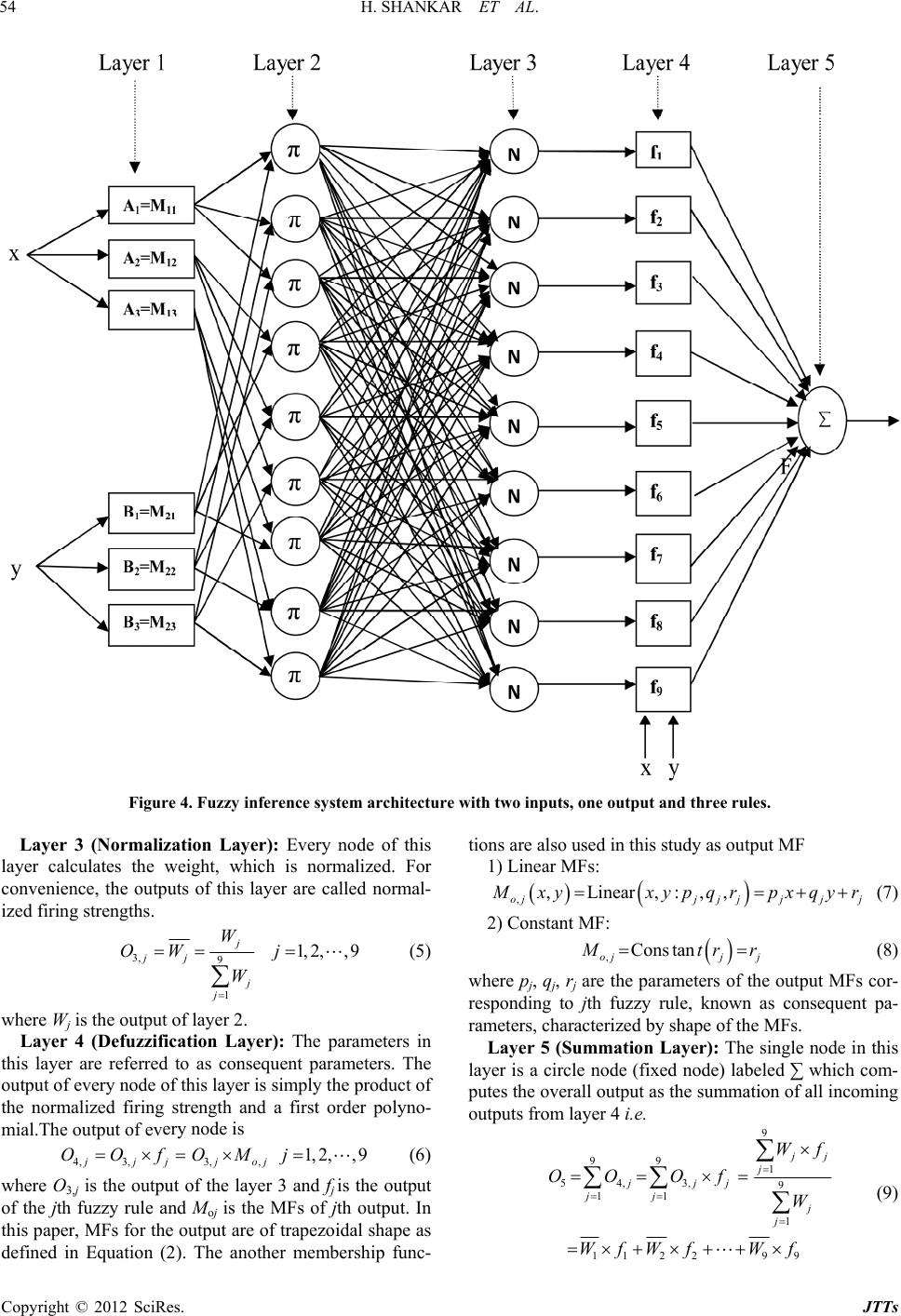

H. SHANKAR ET AL.
54
Figure 4. Fuzzy inference system architecture with two inputs, one output and three rules.
Layer 3 (Normalization Layer): Every node of this
layer calculates the weight, which is normalized. For
convenience, the outputs of this layer are called normal-
ized firing strengths.
3, 9
1
1, 2,, 9
j
jj
j
j
W
OW j
W

 

 (5)
re Wj is the o
ery node is
where O3,j is the output of the layer 3 and fj is the output
of the jth fuzzy rule and Moj is the MFs of jth output. In
of trapezoidal shape as
de
tions are also used in this study as output MF
1) Linear MFs:
whe utput of layer 2.
Layer 4 (Defuzzification Layer): The parameters in
this layer are referred to as consequent parameters. The
output of every node of this layer is simply the product of
the normalized firing strength and a first order polyno-
mial.The output of ev
4, 3,3,,1, 2,, 9 jjjjoj
OOfOMj  (6)
this paper, MFs for the output are
fined in Equation (2). The another membership func-




,,Linear,:,, ojjjjjjj
M
xyxy pqrpxqyr


(7)
2) Constant MF:

,Constan ojj j
M
tr r

 (8)
where pj, qj, rj are the parameters of the output MFs cor-
consequent pa-
Fs.
responding to jth fuzzy rule, known as
rameters, characterized by shape of the M
Layer 5 (Summation Layer): The single node in this
layer is a circle node (fixed node) labeled ∑ which com-
putes the overall output as the summation of all incoming
outputs from layer 4 i.e.
9
99 1
54, 3,9
11
1
112 29 9
j
j
Wf

j
jjj
jj j
j
OO Of
W
WfWf Wf




 
 

(9)

H. SHANKAR ET AL. 55
In this study, all the premise and consequent parame-
teecided in MATLAB tools.
Sugeno Model: The architecture and the fuzzy
soodel is same as that of the Mamdani
mly linear or constan
the output variable. In this study we u
ided in the
M
bines the adaptive learning
capability of Artificial Neural Network (ANN) along with
the intuitive Fuzzy logic (FL) into a single capsule. For a
given input/output dataset, the ANFIS gener
fuzzy inference system (FIS) using grid partiti
nique and membership functions parameters are adjusted
(tuned) automatically until reach the optimal solution
us
rning me-
th
pes of fuzzy reasoning and “if-
th
e optimal solution.
econd interval of time.
Here we judging D/S (Density over Speed ratio), and
estion, namely free flow, slow
taken as the validation data and depends
up
of the model is
ev
match with the
co
ion (10)
rs are manually d
rea-
ning of Sugeno m
odel, but it has ont type of MFs for
se the trapezoidal
MFs for both the inputs (Speed and Density) and con-
stant MFs for the output (LOC). Here also all the premise
and consequent parameters are manually dec
ATLAB tools.
ANFIS Model: Adaptive Neuro-Fuzzy Inference Sys-
tem (ANFIS) is one of the most successful hybrid mod-
eling technique which com
ates the
on tech-
ing either a backpropagation algorithm or in combina-
tion with least squares type method (hybrid lea
od). We use the adaptive neuro-fuzzy inference system
(ANFIS) [17], which use the hybrid learning algorithm
[13] to create rules and adjust membership function pa-
rameters to fit the training data. The membership func-
tions used in ANFIS are gbell’s functions for inputs and
linear functions for output. We train our ANFIS under
100 epochs.
Depending on the ty
en” rules, Sugeno’s fuzzy model, the output of each
rule is a linear combination of input variables plus a con-
stant term or purely constant, because membership func-
tion of output variable are only linear or constant type
and the final output is the weighted average of each
rule’s output. Mamdani Model also has same units as in
Sugeno model, but only difference is that the member-
ship function of output variable may have different type
like trapezoidal, triangulat, Gaussian, exponential etc.
[18]. In our case we chose the trapezoidal membership
function for the output variable (LOC). The ANFIS is
like a fuzzy inference systems, except that here by using
a learning algorithm (either a back propagation alone or
in combination with a least squares estimation) the pa-
rameters of input and output membership function of a
fuzzy inference system constructed by ANFIS, have been
tuned (adjusted) automatically based on the training data
until reach th
4.1. Data Preparation
The road traffic video is recorded by a video camera. The
road traffic video is 90 minutes long taken in the after-
noon (15:07 to 16:37 hours) of February 2, 2011. The
speed of the vehicle is calculated by noting the distance
between two consecutive poles (in the middle of two
lanes i.e. on the divider) that is 24 meters, and also the
travel time of a vehicle between these two poles (Figure
5). And thus the average speed and number of vehicles
(road density) per 20-second and also per 40-second in-
terval of time is collected in the form of matrix. The av-
erage speed and density every 20-second and 40-second
become the input of our fuzzy inference systems (Sugeno
& Mamdani). Another type of input besides vehicle den-
sity and speed, is the human evaluated of congestion
level. By watching the traffic video several times, and we
form a common sense to decide the level of congestion
(LOC) every 20-second and 40-s
evaluate five level of cong
moving, mild congestion, heavy congestion and serious
jam, ranging from “0” to “3”, in which “0” means free
flow and “3” means serious jam. By this way six datasets
are prepared in the form of matrices, in which column 1
is average speed, column 2 is density and column 3 is
LOC (level of congestion), and each dataset contains 68
data pairs (no. of rows), thus we have six 68 × 3 matrix
datasets as:
Dataset I: Average speed, density and LOC every
20-second interval of Lane I (left lane);
Dataset II: Average speed, density and LOC every
40-second interval of Lane I (left lane);
Dataset III: Average speed, density and LOC every
20-second interval of Lane II (right lane);
Dataset IV: Average speed, density and LOC every
40-second interval of Lane II (right lane)
Dataset V: Average speed, total density and LOC eve-
ry 20-second interval of Lane I & Lane II;
Dataset VI: Average speed, total density and LOC eve-
ry 40-seconds interval of Lane I & II.
4.2 Accuracy Assessment
For each input pair (Speed and Density) there is an out-
put value of LOC which is called a data point, the human
evaluated LOC is taken as the standard data of LOC and
depends on the human perceptions, and the model evalu-
ated LOC is
on the adjustment of input/output membership func-
tions of the model. The performance
aluated by a metric, called accuracy which shows how
many output data points of the model
rresponding human evaluated output data points. The
accuracy of the system is defined by Equat


Total DataPointsIncorrectDataPoints
Accuracy TotalData Points

(10)
In addition, to measure how far the incorrect data
points are from the human opinion, another metric is
lled average deviation and is given by ca

H. SHANKAR ET AL.
56
Figure 5. Images taken from traffic video.
AverageDeviation
FuzzyScoreHumanOpinion Score
TotalData Points

 (11)
Human Opinion Score is the LOC rated by human
pioneers, corresponding to each pair of inputs, and Fuzzy
Score is the LOC rated by the fuzzy system, correspond-
ing to the same input pair. The lower value of average
deviation means higher the accuracy of the system and
vice-versa.
Results and Discussions
There are eighteen experiments on LOC evaluat
on the derived parameters described previously, six ex-
periments for each technique. In each experiment, we
va
ut LOC are different for different inference
of congestion (0 - 3) is
ach model, the MFs of
Rule 7: If (Speed is fast) AND (Density is high) then
(LOC is slow moving1);
Rule 8: If (Speed is fast) AND (Density is medium)
then (LOC is free flow2);
Rule 9: If (speed is fast) AND (Density is low) then
(LOC is free flow1).
Experiment I: Average Speed, Density Evaluation of
Lane I, 20-Second by Sugeno Model
Inputs into the Sugeno model are the average speed
e left lane. Here the input MFs are
nd the output MFs are constant type.
Th
and density in th
trapezoidal type a
e range of the speed is between 0 - 60 km/hr and den-
sity range between 0 - 40 vehicles per 20 seconds. The
M
5.
ion based F ranges for average speed are less than 18 km/hr for
slow, 15 - 35 km/hr for medium and more than 30 km/hr
for fast. The MF ranges for density are 0-10 vehicles for
low, 7 - 22 vehicles for medium and more than 18 vehi-
cles for high. The output LO
ry types of input parameters and the evaluation interval.
In all the experiments the membership function ranges
are changed. There are three membership functions of
Speed namely slow, medium and fast, three membership
function of Density namely low, medium and high. The
MFs of outp
C has nine MFs, namely 2
free flow, 2 slow moving, 1 mild congestion, 2 heavy
congestion and 2 serious jam corresponding to the ranges
0, 0.67, 1, 1.33, 1.67, 2, 2.33, 2.67, and 3. First we get
the LOC by manually putting the values of speed and
density in the model and then train this model using AN-
FIS tool using model output as
systems, but the range of the level
same for all the experiments. For e training data and under 80
epochs. ANFIS automatically adjusted MF parameters
and gives better result. Th
output (LOC) are nine in numbers namely—2 free flow,
2 slow moving, 1 mild congestion, 2 heavy congestion
and 2 serious jam. The “if-then” fuzzy rules are applied
on the experiments (Sugeno, 1983), as follows:
Rule 1: If (Speed is slow) AND (Density is high) then
(LOC is serious jam1);
Rule 2: If (Speed is slow) AND (Density is medium)
then (LOC is serious jam2);
Rule 3: If (Speed is slow) AND (Density is low) then
(LOC is heavy congestion1);
Rule 4: If (speed is medium) AND (Density is high)
then (LOC is heavy congestion2);
Rule 5: If (Speed is medium) AND (Density is me-
dium) then (LOC is mild congestion)
Rule 6: If (speed is medium) AND (Density is low)
then (LOC is slow moving2);
e MFs and Fuzzy rules, and 3D
surface are shown in Figure 6.
The list of output LOC for every data pair is shown in
the Table 1. The human evaluated values and model ba-
sed LOC values are closely matching with respected to
the given input variables. The difference of 0.20 in val-
ues of LOC is considered as acceptable error for conven-
ience (0.20 is about 7% of LOC range). The MFs above
yield the accuracy of 55.88%, and average deviation of
0.0426323 levels.
Experiment II: Average Speed and Density Evalua-
tion of Lane II, 20-Second by Sugeno Model
In a 20 second evaluation interval and Sugeno-type
inference system, inputs fed into the system i.e. average
speed and density of the right lane. The model is trained

H. SHANKAR ET AL. 57
Figure 6. MATLAB program showing the MFs and fuzzy rule, and 3D surface of the model.
Table 1. Comparative table of human evaluated vs model Loc.
Average Speed
(km/hr) Density (No. of vehicles) LOC (Density/Speed)*3 Human Opinion LOC Model LOC Time
40 10 0.45 0.45 0.67 15:07:07
25 7 0.84 1.1 1.33 15:09:13
28 4 0.43 1.1 1.33 15:11:52
12 10 2.50 2.85 *2.67 15:15:00
16
···
···
···
14
···
···
2.68
···
···
2.1
···
···
*2.2
···
···
15:15:40
···
···
··· ··· ··· ··· ···
by ANFIS under same conditi
above MFs yield the accuracy of 70.68%
de 01838
Ex Id and-
tion of I, 40-Second by Sugeno Model
Similarly, a 40-secondaluation interval augeno-
type inference system issted with averagd and
density lane. The ge of the speed iseen 0 -
60 km/hr and density ra between 0 - 60 ve
40 seco and the rang LOC is 0 - 3.
The ges of the MFf density are 0 - hicles
for low - 35 vehicler medium and mthan 30
ehicles for high, and the average speed and output MF
of 57.35%, and average
de
ink that the
ev
Speed and Density Evalua-
by Sugeno Model
ondtion intervaliven into the
systeng with e speed and dey of the right
lane. All inputs, ou, fuzzy ruleFs (shape,
and ns) are thee as those ient I, and
ranged training eters are sa experiment
III. Here we again want to see the effect of evaluation
interval
The MFs yield thcuracy of 55.88%, and the aver-
age dtion of 0.0117 levels. Therformance is
not better than that of experiment II, h leads us to
think that, it is not necessary that the evaluation interval
no Model
ons as in experiment I. The
and average
Experiment IV: Average
tion of Lane II, 40-Second
viation of 0.0
periment II2 levels. : Average Spee Density Evalua
Lane
evnd S
tee spee
of leftran betw
ngehicles per
nds,e of
rans o20 ve
, 15s foore
v
ranges are same as in experiment I. The model is trained
by ANFIS under same conditions as in experiment I. The
MFs above yield the accuracy
viation of 0.0600294 levels. This performance is better
than that of experiment I, which leads us to th
aluation interval may affect the performance of the
fuzzy inference system.
may affect the performance of the fuzzy systems.
Experiment V: Average Speed and Total Density Eva-
luation of Lane I & II, 20-Second by Suge
Here, 40-sec
m alo
evalua
averag
is g
nsit
tputss, and M
ame samn experim
s anparamme as in
on level of congestion.
e ac
evia634is p
whic
In this experiment, evaluation interval is reduced to
20-second, and inputs into the model are the average
speed and total density of both the lanes. The MFs yield
the accuracy of 67.65%, and the average deviation of

H. SHANKAR ET AL.
58
0.1573970 levels.
Experiment VI: Average Speed and Total De nsi ty Eva-
luation of Lane I & II, 40-Second by Sugeno Model
In this experiment, we assume 40 second evaluation
interval with inputs average speed and total density of
both the lanes into the system. All inputs, outputs, fuzzy
ru
xperiment
is
s evaluation interval in-
cr
stem is
us
ne.
H
18 km/hr for slow, 15 - 35 km/hr for
m
for
m
les and MFS (shape, and names) are the same as those
in experiment I. Average speed range in the e
same as experiment I, and we have changed the range
of total density to 0 - 80. The MF ranges of total density
are low (below 22 vehicles), medium (18 - 40 vehicles)
and high (above 35 vehicles). The MFs yield the accu-
racy of 72.05%, and the average deviation of 0.1564117
levels. Here, the evaluation interval improves the accu-
racy of the model, it means a
eases, accuracy of the model also increases and vice-
versa.
Experiment VII: Average Speed and Density Evalua-
tion of Lane I, 20-Second by Mamdani Model
In this experiment, Mamdani-type inference sy
ed with 20-second evaluation interval. Inputs into the
system are the average speed and density of left la
ere the input MFs are trapezoidal type and the output
MFs are also trapezoidal. The range of the speed is be-
tween 0 - 60 km/hr and density range is between 0 - 40
vehicles per 20-seconds. The MF ranges for average
speed are less than
edium and more than 30 km/hr for fast. The MF ranges
for density are 0 - 10 vehicles for low, 8 - 22 vehicles
edium and more than 19 vehicles for high. The output
level of congestion has nine members, namely 2 free
flow, 2 slow moving, 1 mild congestion, 2 heavy conges-
tion and 2 serious jam corresponding to the ranges below
0.65, between 0.55 - 1.25, 1.15 - 1.85, 1.75 - 2.45 and
above 2.35. The LOC is obtained by manually putting the
values of speed and density in the model (in rule viewer)
and then compare with the human evaluated LOC. In
Figure 7, shows the MFs of input/output variable and
Fuzzy Rule viewer, and 3D surface of the model. The
MFs above yield the accuracy of 82.35%, and the aver-
age deviation of 0.1115213 levels.
Experiment VIII: Average Speed and Density Eva-
luation of Lane II, 20-Second by Mamdani Model
In this experiment, Mamdani-type inference system is
used with 20-second evaluation interval, and inputs into
the system are the average speed and density in the right
lane. All inputs, output, fuzzy rules, and MFs (shape,
ranges and names) are the same as those in experiment
VII. The MFs above yield the accuracy of 83.82%, and
the average deviation of 0.0917643 levels.
Experiment IX: Average Speed and Density Evalua-
tion of Lane I, 40-Second by Mamdani Model
In this experiment, a 40-second evaluation interval,
and inputs into the system are the average speed and den-
sity in the left lane. All inputs, output, fuzzy rules, and
MFs (shape, and names) are the same as those in experi-
ment VII. The ranges of input speed and output LOC and
their MFs are same as those of experiment VII. The
range of density between 0 - 60 vehicles per 40 seconds
and the ranges of MFs of density are, below 20 for Low,
between 15 - 35 for Medium and above 31 for High. The
MFs above yield the accuracy of 77.94%, and the aver-
age deviation of 0.1112561 levels. This performance is
not better than that of experiment VII, which infers that it
is not necessary that the evaluation interval could im-
prove the accuracy of the Mamdani-type fuzzy inference
system.
Figure 7. MATLAB program showing MFs and fuzzy rules, and 3D surface of the model.

H. SHANKAR ET AL. 59
Experiment X: Average Speed and Density Evalua-
tion of Lane II, 40-Second by Mamdani Model
In this experiment, under similar conditions of ex-
periment IX, the MFs yield the accuracy of 73.52%, and
the average deviation of 0.1441361 levels. This per-
formance is not better than that of experiment VIII, wh-
ich again leads to think that it is not necessary that the
evaluation interval could improve the accuracy of the
Mamdani-type fuzzy inference system.
Experiment XI: Average Speed and Density Evalua-
tion of Lane I & II, 20-Second by Mamdani Model
In this experiment, Mamdani-type inference system is
used with 20-second evaluation interval, and inputs into
the system are the average speed and density of both the
lanes. All inputs, output, fuzzy rules, and MFs (shape, and
names) are the same as those in experiment VII. The
ranges of inputs and output LOC and their MFs of are
same as those of experiment IX. The MFs above yield
of
.
Experiment XIII: Average Speed and Density Eva-
luation of Lane I, 20-Second by ANFIS Model
ANFIS model is deployed with the three gbell’s MF
for each input, and nine linear MF for the output. The
ranges of each variable are automatically decided by us-
ing grid Partition technique using Matlab ANFIS tools.
Inputs into the system are the inputs average speed, den-
sity and output human opinion LOC of left lane in the
form of a matrix (dat.file). The input-output dataset are
then passed through the ANFIS tool for learning and
automatically adjusting the output. After 100 epochs, and
using hybrid learning algorithm, the automatically gener-
ated FIS is trained, and thus the ANFIS is ready to
evaluate the congestion status. The ANFIS outputs after
training,model and structure are shown in Figure 8(a)
and (b). The MFs above yields the accuracy of 72.05%,
and the average deviation of 0.0005667 levels.
Experiment XIV: Average Speed and Density E
odel the accuracy
0
64.70%, and the average deviation of luation of Lane II, 20-Second by ANFIS M
1756654 levels
Experiment XII: Average Speed and Density Evalua-
tion of Lane I & II, 40-Second by Mamdani Model
This experiment is deployed with Mamdani-type in-
ference system with 40-second evaluation interval, and
inputs into the system are the average speed and density
of both the lanes. All inputs, output, fuzzy rules, and
MFS (shape, and names) are the same as those in ex-
periment VII. The ranges of input speed and output LOC
and their MFs are same as those in experiment VII. The
range of density between 0 - 60 vehicles per 40 seconds
and the ranges of membership functions of density are,
below 22 for Low, between 18 - 40 for Medium and
above 35 for High. The MFs above yield the accuracy of
63.23%, and the average deviation of 0.1867251 levels.
This performance is not much better after increasing the
evaluation interval for both the lanes. Again it is not clear
that evaluation interval could improve the performance
of the model.
va-
In this experiment, we repeat the same procedure as in
experiment XIII, but the input-output dataset of left lane
is loaded into the ANFIS tool.
The MFs above yield the accuracy of 80.88%, and the
average deviation of 0.0870766 levels.
Experiment XV: Average Speed and Density Evalua-
tion of Lane I, 40-Second by ANFIS Model
In this experiment, we repeat the same procedure as in
experiment XIII, but the evaluation interval increases
from 20 seconds to 40 seconds, and input-output dataset
of left lane is loaded into the ANFIS tool. The MFs
above yields the accuracy of 88.23%, and the average
deviation of 0.0109558 levels. This performance is better
than that of experiment VII, which leads to think that the
evaluation interval may affect the performance of the
ANFIS.
Experiment XVI: Average Speed and Density Eval-
uation of Lane II, 40-Second by ANFIS Model
In this experiment, we repeat the same procedure as in
(b) (a)
Figure 8. (a) Training and FIS output; (b) ANFIS model str ucture .

H. SHANKAR ET AL.
60
experiment XV, but input-output dataset of right lane is
loaded into the ANFIS tool. The MFs yield the accuracy
of 77.94%, and the average deviation of 0.0018514 levels.
This performance is impressive than that of experiment
could im
XIV, which leads to think that it is not necessary that the
evaluation interval could improve the accuracy of the
ANFIS.
Experiment XVII: Average Speed and Total Density
Evaluation of Lane I & II, 20-Second by ANFIS Model
In this experiment, we repeat the same procedure as in
experiment XIII, but the input-output dataset of both the
lanes is loaded into the ANFIS tool. The MFs yield the
accuracy of 73.52%, and the average deviation of 0.0018
661 levels.
Experiment XVIII: Average Speed and Total Density
Evaluation of Lane I & II, 40-Second by ANFIS Model
In this experiment, the same process is repeated as in
experiment XIII and XVII, but the evaluation interval
increases from 20-second to 40-second. The
uracy of 72.05
prove the performance of ANFIS. Table 2 sum-
m
model is higher than the manually tuned Mamdani and
Sugeno model. However, the accuracy achieved by
manually tuned Mamdani and Sugeno model is very near
to that of ANFIS model, which shows that fuzzy infer-
ence systems can capture the human perceptions as well.
Overall the maximum accuracy achieved by Sugeno
model is 72.05%, Mamdani model is 83.82% and ANFIS
model is 88.23%. These models are also applied after
changing the evaluation interval of each lane individually
and combination of both and evaluate the accuracy of the
models. For left lane, as the evaluation interval increases
from 20 seconds to 40 seconds then the accuracy of
Sugeno model increases from 55.88% to 57.35%, but the
ame time accuracy of Mamdani model reduces
nd the accuracy of ANFIS model
3%, which shows that it is
f m
rs
MFs above 82.35% to 77.94% a
yield the acc%, and the average deviation increases from 72.05% to 88.2
reach to 0.0003088 levels. This performance is not again
very impressive after increasing the evaluation interval.
Therefore, it is not conclusive that evaluation interval
Table 2. Summary o
Experiment No. Fuzzy System Input par amete
arizes the accuracy and average deviation of all the
above experiments.
In most of the cases the accuracy achieved by ANFIS
s from
not necessary that evaluation interval could improve the
accuracy of the model. Also for right lane as the evalua-
tion interval increases from 20 seconds to 40 seconds, the
odel performance.
Evaluation Interval Accuracy Average deviation
I Sugeno-type Avg.Speed, Density of left lane 20 seconds 55.88% 0.0426323
II Sugeno-type Avg.Speed, Density of right lane
e
th l
th l
e
e
th l
h l
XIII ANFIS
Avg.Sp
20 seconds 70.58% 0.0018382
40 seconds 57.35% 0.0600294
40 seconds 55.88% 0.0634117
anes 20 seconds 67.65% 0.1573970
anes 40 seconds 72.05% 0.1564117
20 seconds 82.35% 0.1115213
20 seconds 83.82% 0.0917643
40 seconds 77.94% 0.1112561
40 seconds 73.52% 0.1441361
anes 20 seconds 64.70% 0.1756654
anes 40 seconds 63.23% 0.1867251
III Sugeno-type Avg.Speed, Density of left lane
IV Sugeno-type Avg.Speed, Density of right lan
V Sugeno-type Avg.Speed, Total Density of bo
VI Sugeno-type Avg.Speed, Total Density of bo
VII Mamdani-type Avg.Speed, Density of left lan
VIII Mamdani-type Avg.Speed, Density of right lane
IX Mamdani-type Avg.Speed, Density of left lane
X Mamdani-type Avg.Speed, Density of right lan
XI Mamdani-type Avg.Speed, Total Density of bo
XII Mamdani-type Avg.Speed, Total Density of bot
eed, Density and Human opinion LOC o
f
left laneconds 72.05% 0.0005667
Avg.Speed, Dinion LOC o
e 20 s
f
XIV ANFIS ensity and Human op
right lane
X opinion LOC o
20 seconds 80.88% 0.0870766
V ANFIS
Avg.Speed, Density and Human
f
left lane
X pinion LOC o
40 seconds 88.23% 0.0109558
VI ANFIS
Avg.Speed, Density and Human o
f
right lane
Avg.Speed, Total Density and
40 seconds 77.94% 0.0018514
XVII ANFIS Human opinion20 seconds 73.52% 0.0018661
XVIII ANFIS an opinion
LOC of both lanes 40 seconds 72.05% 0.0003088
LOC of both lanes
Avg.Speed, Total Density and Hum

H. SHANKAR ET AL. 61
accuracy of Sugeed
55.88%, accuracy of Mamdani model decreases from
83.82% 73.52%f
from 8% to 77rl
both the lanes, the accuracy Suge
from 5% to 7r
decrearom 643
FIS mel decrea.5
again shows that it is
val coproven
6. Conclusions
In this study, we prophe a of fuzzy infer-
ence system (Sugeno-type, Mam
neuro-fuzzy inference system)
the lestion. Basically the level of
congestion (LOC) offi
able to express the situation frolow to serious
traffi The perfo of
evaluated by measuring accurac
an n. Througent e
interval
cy, but this effect depends on nature
articular road segment and particular
Practical applications of Research,” US Department of
Commercen DC,
D. Branston, Fun
portation Rl. 10, 76, p
doi:10.1016 (76)90
no model ruced from 70.58% to
to, and that oANFIS model decreases
[2]
0.88.94%. Similay for the combination of
of
2.05%, accu
no model increases
acy of Mamdani model 67.6
ses f.70% to 63.2%, and that of the AN-
odses from 73
not necessary t
2% to 72.05%, which
hat evaluation inter-
uld im the performace of the model.
osed tdvantage
dani-type and adaptive
technology, to evaluate
vel of road traffic conge
road trafcs is a continuous vari-
m free f
c jam.rmanceour proposed systems is
y of outputs against hu-
xperiments, we find that mopinioh differ
the manually tuned fuzzy inference system achieve the
accuracy which is very near to the accuracy achieved by
adaptive neuro-fuzzy inference system. It means the
fuzzy inference system can capture the human expertise
better than manual adjustment of input/output member-
ship functions. Two types of fuzzy logic inputs- average
speed and density within an interval. We investigate the
effect of using single lane traffic information as opposed
to two lane information. It is also observed that how the
evaluation interval affects the accuracy of the system.
The results are not conclusive whether longer
can improve accura
of traffic flow at p
time. The systems used in this study have advantage of
minimum requirement of input data, and better accuracy
and reduced error margin. Therefore, it is possible to use
fuzzy system to evaluate the road traffic congestion with
greater accuracy and low error margins. However, accu-
racy of fuzzy systems depends highly on the types of
rules, and how the rules are defined along with member-
ship function ranges.
Future Scope: In general, the congestion is the re-
striction in the movement of the vehicles on the roads,
therefore it can be compared with the impedance of the
roads which can be used in the network analysis in GIS.
In addition to that, congestion can be evaluated for dif-
ferent times and thus temporal impedance can be calcu-
lated which can be used in temporal network analysis.
REFERENCES
[1] Bureau of Public Roads, “Highway Capacity Manual:
, Washingto 1950.
“Link Capacity
esearch, Vo
ctions: A Re
No. 4, 19
view” Trans-
p. 223-236.
/0041-1647 055-1
[3] P. Posawang,ard, W.
Atikom, “Pased Rfic Colas-
sification Ual NetProcethe
World Congress on Engineering
[4] A. P. Addepalli, “Study of Mraffic ac-
teristics: Ac Simulation Approachm,” M.Tech
Thesis, IIT, Mad.
C.-C. Lee, ic in Cstemgic
ller ransac Syste
Cyberneticso. 2, 1 404-4
110
S. Phosa
erception-B
Polnigongit and W
oad Traf
. Pattara-
ngestion C
sing Neurworks,”
, London, 1-3
edings of
July 2009.
ixed TFlow Char
Microscopi
ras, 2000
[5] “Fuzzy Logontrol Sys: Fuzzy Lo
ControI,” IEEE T
, Vol. 20, N
tions on
990, pp.
ms, Man and
18.
doi:10. 9/21.52551
[6] C.-C. L
Contro
ee, “Fuzzy Logic in Control Systems: Fuzzy Logic
ller ransa Syst
etics, Vol. 20, No. 2, 1990, pp. 419-435.
II,” IEEE Tctions onems, Man and
Cybern
doi:10.1109/21.52552
[7] A. Kablan,Neuroferen
Financial Tng Intason
odel ademy ce, En
Technology o. , 2079-48
“Adaptive
rading Usi
-Fuzzy In
raday Se
ce System for
ality Observa-
tion M,” World Ac
, Vol. 58, N
of Scien
09, pp. 4
gineering and
8.
[8] F. Porikli and X. Li, “Traffic Congestion Estimation Us-
ing HMM Models without Vehicle Tracking,” IEEE In-
telligent Vehicles Symposium, Parma, 14-17 June 2004,
pp. 188-193. doi:10.1109/IVS.2004.1336379
[9] W. Pattara-Atikom and P. Pongpaibool, “Estimating Road
Traffic Congestion Using Vehicle Velocity,” Proceeding
of 6th International Conference on Telecommunications,
Chengdu, June 2006, pp. 1001-1004.
[10] B. Krause and C. von Altrock, “Intelligent Highway by
Fuzzy Logic: Congestion Detection and Traffic Control
on Multi-Lane Roads with Variable Road Signs,” 5th In-
ternational Conference on Fuzzy Systems, New Orleans,
8-11 September 1996, pp. 1832-1837.
doi:10.1109/FUZZY.1996.552649
[11] A. S. Alfa, “Understanding Urban Traffic Congestion dur-
ing Peak Periods,” Proceedings of International Confer-
ence on Road and Road Transport Problems (ICORT-88),
Roorkee, 12-15 December 1988, pp. 518-527.
[12] L. Jia and C. Li, “Congestion Evaluation from Traffic
Flow Information Based on Fuzzy Logic,” IEEE Intelli-
gent Transportation Systems, Vol. 1, 2003, pp. 50-53.
[13] P. Mitra, “ANVoltage Regulator
with Hybrid Learning Algorithal Journal
daptive Neuro-Fuz-
ment, Vol. 4, No. 1,
FIS Based Automatic
m,” Internation
of Advances in Soft Computing and Applications, Vol. 2,
2010.
[14] S. M. Seyedhoseini, “Application of A
zy Inference System in Measurement of Supply Chain
Agility: Real Case Study of a Manufacturing Company,”
African Journal of Business Manage
2010, pp. 83-96.
[15] T. O. S. Hanafy, “A Modified Algorithm to Model Highly
Nonlinear System,” Journal of American Science, Vol. 6,
No. 12, 2010, pp. 747-759.
[16] T. Takagi and M. Sugeno, “Derivation of Fuzzy Control
Rules from Human Operator’s Control Actions,” Pro-

H. SHANKAR ET AL.
62
ceedings of IFAC Symposium on Fuzzy Inform
2005.
d
ation, Transactions on Systems, Man and Cybernetics, Vol. 3,
No. 1, 1973, pp. 28-44.
[19] N. Patchanee, P. Tangamchit and P. Pongpaibool, “Roa
Knowledge Representation and Decision Analysis, Mar-
seilles, 19-21 July 1983, pp. 55-60.
[17] A. P. Paplinski, “Adaptive Neuro-Fuzzy Inference S
tem (ANFIS),” 20 May
ys- T
[18] L. A. Zadeh, “Outline of a New Approach to the Analysis
of Complex Systems and Decision Processes,” IEEE
raffic Estimation from a GPS-Equipped Car Using Fuz-
zy Logic,” Proceeding of 29th Electrical Engineering Con-
ference, Chonburi, 9-10 November 2006, pp. 1081-1084.