ABSTRACT

The application herein involves the optimal management of renewable and nonrenewable resources within the context of a stochastic model of optimal control. By characterizing the two dimensional Bellman solution, three rules with respect to resource management are established. Within the context of coastal development, this analysis may help to explain why renewable resources may become increasingly vulnerable to random external shocks as nonrenewable resources are depleted. Although existence of an optimal closed form solution to the multi-sector Bellman model remains an open mathematical question, this analysis offers a characterization which can be applied to other scenarios in economics or finance in which two assets following stochastic processes interact.

1. Introduction

Dynamic programming, or optimal control theory, has been useful in helping economists to model dynamic change within various systems or applications. Most of the applications have employed deterministic methods of optimal control. Though this is helpful in understanding expected long-run outcomes, a more thorough understanding of how systems behave requires a stochastic analysis. Stochastic optimal control would be an ideal methodology, but it has not been thoroughly exploited due to the absence of a universal closed form solution to the multi-dimensional stochastic optimal control problem. This paper provides a method for characterizing the solution to the two-dimensional stochastic dynamic programming problem while examining the link between nonrenewable and renewable resource management.

2. Application to Coastal Development

Since the 1960’s, there has been much discussion concerning the management of our natural resources. Most scenarios involve a fundamental trade-off, whether it be the impact on coastlines from offshore oil drilling, the effect on wildlife of a pipeline from Canada to the Gulf of Mexico, or the consequences of new construction near a coastal estuary. This suggests a rather fundamental economic problem. That is, what are the optimal extraction rates of dependent renewable and exhaustible resources when extracting one of the resources may negatively impact the other?

Hotelling [1] was the first to mathematically model optimal management of a nonrenewable resource, and Dasgupta and Heal [2], among others, have expanded upon Hotelling’s work. In contrast to nonrenewable resources, associated with each renewable resource is a renewal (or spawning) function [3,4]. The interdependence of nonrenewable and renewable resources can be displayed through this spawning function. For example, coastal development can be characterized as the extraction of a nonrenewable resource (undeveloped land) and its effect on a renewable resource (the indigenous fish or wildlife). Extraction of this resource eliminates natural habitats and increases pollution levels. As a result, development can prove detrimental to the spawning rates of wildlife by contributing to loss of habitat, disease or sterilization. Although less likely, a decline in fish or wildlife may also reduce the desire to further develop a coastal area. Finally, severe weather and unpredictable catastrophic events such as oil spills influence natural resource stocks and thus the optimal rates of harvest or extraction. Therefore, uncertainty is also an important consideration.

3. Methodology

Merton [5,6], Fischer [7], and Pindyck [8] provide significant insight in their study of financial assets using (one-dimensional) stochastic optimal control. Both deterministic and stochastic optimal control have been particularly useful in developing a theoretical foundation for the study of resource management. In particular, Swallow [9] studies the effect extraction of a nonrenewable resource has on a renewable resource employing deterministic optimal control. Depletion of the nonrenewable resource is assumed to have an adverse effect on the renewal rate (spawning rate) of the renewable resource. The two types of resources interact through this rate of renewal. However, Swallow’s model has its limitations. The model does not allow for joint maximization of the harvest and extraction rates, and it is deterministic. Pindyck [10] uses stochastic optimal control to model the optimal extraction of a single nonrenewable resource when demand for the resource, as well as its reserve supply, follow stochastic Ito processes. Although Pindyck begins his analysis within a global framework, the inability to derive a closed form solution forces him to take expected values, thereby localizing his results around a mean optimal rate of harvest. This essentially hides, or smooths-out, the stochastic element. Chen and Insley [11] consider regime switching in a forestry model. The optimal harvest rate is determined by the value of lumber. The value of lumber is estimated via a stochastic Bellman process. The Bellman equation has frequently been used to estimate real options pricing in finance [12]. Insley and Rollins[13] use this approach, modeling the optimal harvest rate of lumber as a call option that can be exercised at any time. Theirs is a one dimensional Markov decision process model which is solved through empirical simulation.

In contrast, this paper provides a general characterization of the solution to a stochastic version of the tworesource Swallow model using the methods of stochastic optimal control. In the most general version of our model, society acts to maximize expected discounted utility over an infinite time horizon, subject to two laws of motion. We examine the effect extraction of the exhaustible resource has on the optimal harvest rate of the renewable resource. This effect is transmitted by the renewal (or spawning) function. In the spirit of Swallow’s model, we adopt the paradigm of examining the effects of coastal development on an estuary. In this context we consider marine life to be the renewable resource and undeveloped coastal real estate to be the nonrenewable resource. It is assumed that although development benefits society by providing jobs and a higher standard of living, it also produces negative externalities, damaging the marine life within the estuary.

The remainder of the paper is presented as follows. Section four extends the deterministic model in [9] to the stochastic case. In section five, the optimal harvest and extraction rates for the two natural resources are derived, and in the spirit of [1], [14] and [15] a stochastic “golden rule” describing the opportunity costs associated with consuming the resources is described. Society’s preferences are revealed by the optimal extraction rates of the resources. Section six concludes the paper, and the final section contains a mathematical appendix.

4. The Model

The methods of optimal control are used to determine the optimal extraction rates of the natural resources. The model consists of an intertemporal social welfare function which is maximized subject to two stochastic, dynamic constraints, or laws of motion. One characteristic of using the methods of optimal control is that the optimal solution is time consistent. It has the property that all future decisions depend only on the initial stocks, and these stocks are updated with the passage of time. The optimal solutions reflect this “feedback control”¹. The relevant variables and their arguments are defined in the following manner.

4.1. Definitions

existing stock of the renewable resource at time t, with initial stock,.

stock of the nonrenewable resource at time t, with initial stock,.

rate of extraction of the renewable resource, or the harvest rate.

rate of extraction of the exhaustible resource, or the development rate.

exogenous rate of renewal of the renewable resource, or spawning rate.

Intuition suggests that is increasing and convex in both X and E. That is, I assume are all positive. I also assume that X and E are complementary in the sense that increases with X and increases with E. Thus,. Explicitly stated, one must find h and b satisfying the following value function.

(P)

subject to the stochastic Itô processes for X and E:

and          (L1)

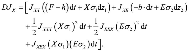
. (L2)

is the present value form of the value function, or indirect utility function. Assume is differentiable to the third order in each variable. With respect to the laws of motion, and are two standard Wiener processes, the continuous time analogue of the random walk. Thus, the instantaneous net growth rate of the renewable resource has mean, or ‘drift,’ equal to and variance. The instantaneous exploitation rate of the nonrenewable resource has drift, and variance,. If instead, (L1) were written in terms of relative change, , then the initial stock could not be exhausted in finite time [17,18]. As written, this is intuitively appealing for it suggests that society has the distinct ability to eventually eliminate the resource.

4.2. Preliminary Results

Lemma 1: The optimal control problem (P) with respect to and must necessarily satisfy the present value form of the Bellman equation,

(1)

Proof. Located in Appendix. ■

The solution to the natural resource problem can be obtained by solving the stochastic Bellman Equation (1). The first order conditions for the maximum are determined by differentiating the current value form of the Bellman function,

(2)

with respect to the control variables h and b [19]. The first order conditions for the maximum are: and. By [20], concavity assumptions on imply that, at optimal h and b,

(3)

The second order condition for a maximum requires the hessian to be positive semi-definite [21]. That is, the determinant of the hessian must be positive, or.

The concavity assumption insures that are negative. Since U is assumed to be at least twice continuously differentiable with the second derivative continuous,. Since intuition suggests that the marginal utility derived from harvesting an additional unit of marine life should increase with additional development, assume. For example, development clearly affects utility derived from marine life (one will enjoy the fruits of the sea more if they have a nice, warm, comfortable place to stay at night). In addition, intuition from our example supports the assumptions,.

If and are solutions to the problem (P) with respect to (L1) and (L2) as determined by the Bellman Equation (2), then is the optimal harvest rate for the renewable resource and is the optimal extraction rate for the nonrenewable resource. In other words, in order to derive the expressions for the optimal harvest rate of the renewable resource and the optimal extraction rate of the nonrenewable resource, one must solve (2’),

(2’)

Then, solutions and yield the maximum.

The optimal Bellman equation satisfies Equation (2) without the “max”,

This equation holds only for the optimal values, and. Thus, for expositional convenience, one may assume without confusion that Thus, the optimal Bellman equation becomes:

(4)

Defining the shock term to be:

Equation (4) becomes,

(4’)

The trick in solving for the optimal harvest rate of the renewable resource, h, is to first differentiate the Bellman equation with respect to each of the state variables. These equations reflect changes in the solution in response to incremental changes in stocks.

Lemma 2. The Bellman stock derivatives are:

1) Renewable Resource:

(5a)

with renewable resource shock

2) Nonrenewable Resource:

(5b)

with nonrenewable resource shock

Proof. Located in Appendix.

5. A Stochastic Golden Rule

Theorem 1. The optimal harvest rate for the renewable resource is:

Proof. Using (5a) and (5b) one can solve for the optimal rates, h and b. Obtain the optimal harvest rate by solving (5a) for b, and then substituting this expression into (5b). ■

Note that the denominator is the determinant of the hessian of J. That is,. Lettingone can rearrange the optimal harvest rate equation in the following manner:

(6)

Dissecting this equation intuitively, an obvious result is that the optimal harvest rate is directly related to the spawning rate. Changes in the spawning rate, F, lead to changes in the harvest rate, h, of the same magnitude and direction. Also note that Equation (6) contains and which represent the marginal changes in the spawning rate from changes in the resource stocks. is the shadow price of the renewable resource. The impact the shadow price has on the on the harvest rate is mitigated by the discount rate as well as by changes in the spawning rate. and indicate that the extent to which the shadow price affects the harvest rate depends on the sensitivity of the spawning function to existing resource stocks. For example, if development has a particularly detrimental impact on the spawning rate (is large), then the optimal harvest rate will be lower for any given shadow price of the renewable resource.

Similarly, and represent the sensitivity of the shocks to changes in the natural resource stocks. If is large, then even small changes in E or X respectively will exacerbate the effect of the shock. Similarly, if is small, then the resource stocks have little effect on the shocks. Finally, as expected, increases in lead to increases in h; for the more society discounts the future the less it will conserve.

In order to analyze this expression further it is necessary to know the signs of the coefficients and . Unfortunately, these signs depend on the signs of the higher order derivatives of the value function and there is currently no mathematical algorithm for which the value function can be determined in general. However, for many reasons it is “natural” to focus on the case where is positive and is negative2.

To begin with when an increase in the discount rate unambiguously leads to a corresponding increase in the optimal harvest rate. Likewise a decrease in will cause h to decline. Thus, if society heavily discounts the future it is less concerned with making certain that future generations will be able to enjoy the resource. As a result, society will opt for a relatively high rate of harvest.

Note that whenever, the impact of both on the harvest rate is negative. Thus, the more sensitive the shocks are to changes in the stocks, the lower the harvest rate. This represents a “precautionary motive” on the part of society. If uncertainty is exacerbated by changes in the resource stocks then it is wise to extract the resources at a slower rate.

Corollary 1. The stochastic golden rule for harvesting the renewable resource is³

(6’)

Proof. This follows directly from Equation (6). ■

Equation (6) states that the returns to consumption exactly balance the returns to conservation. The returns to consumption, on the left hand side, involve F and ρ. The spawning function is present because consuming the renewable resource still leaves society with the offspring of whatever stock remains. Also, one can see that the term involves a weighted difference of the shadow prices of the resources. The higher the difference in shadow prices, the more influence the discount rate has in driving up the optimal harvest rate. Thus, is the marginal return to consumption. The right hand side represents the returns to conserving the single period quantity, h. The remainder of this side of the expression contains the values of the marginal spawning rates, the value of the offspring that is gained by not consuming h, and the shock terms. The term involving the difference in the shocks can be interpreted as the “smoothing” that comes about through conservation.

Theorem 2. The optimal extraction rate for the nonrenewable resource is:

(7)

Proof. Solve (5a) for the optimal harvest rate and substitute this expression into (5b) to get the optimal extraction rate of the nonrenewable resource. ■

Next, let

then one can rewrite (7) as:

(8)

For the same reasons detailed above, it is most reasonable to investigate the case where. Equation (8) illustrates the relationship between the two natural resources. The analysis is similar to the analysis of the optimal harvest rate. The shock terms influence the optimal extraction rate of the nonrenewable resource and the renewable resource in similar fashion. Once again the discount rate is positively related to the extraction rate of the natural resource. However, by extracting the nonrenewable resource society forgoes the potential value of the additional progeny associated with the marginal spawning rate. Simply put, by decreasing the stock of the nonrenewable resource and fall. Thus, the value associated with the offspring is lower (by) than it would have been if the nonrenewable resource had been conserved. Therefore, extraction of the nonrenewable resource is a detriment to the spawning ability of the renewable resource. This is the method by which the externality is revealed.

Corollary 2. The Golden Rule for the extraction of the nonrenewable resource is:

(9)

Proof. The proof follows directly from Equation (8). ■

As with the golden rule for the renewable resource, this equates the return to consumption with the return to conservation.

Equations (5a) and (5b) also suggest an alternative approach to analyzing the relationship between renewable and nonrenewable resources. Now, set Equation (5a) equal to Equation (5b). An alternative expression for the optimal harvest rate is:

(10)

Of course, one could also use this to solve for an alternative optimal extraction rate. However, note that by the first order conditions (3). Thus, the expression, , is the net shadow price or net marginal social value of the natural resources. Let, then, and. One can rewrite (10) as,

(11)

Now it is possible to solve for the optimal development rate,

(12)

Expression (12) is the optimal extraction rate function for the nonrenewable resource in terms of the harvest rate associated with the renewable resource.

Use this approach to investigate the relationship between the harvest and extraction rates. In order to accomplish this, it is necessary to examine the coefficients of (11) and (12). If, then, and the marginal unit of a unit of the nonrenewable resource (land) is worth more to society than the marginal unit of the renewable resource (marine life). Also, by the first order condition (3) it then follows that, and the marginal utility associated with development is greater than the marginal utility associated with harvesting marine life. Thus, a society where is more interested in enhancing its ability to develop (extract the nonrenewable resource). In contrast, if then society will be more interested in improving its ability to harvest the marine life within the estuary (harvest the renewable resource). For example, a society with an abundance of undeveloped land is able to sustain a relatively high rate of development. Thus, may be relatively low compared to, so and this society would be most interested in enhancing its capacity to harvest the estuary. A society rich in the renewable resource would find that. This society would increase its utility the fastest if it were able to develop coastal property. As increases, society increasingly desires the nonrenewable resource over the renewable resource. Alternatively, as decreases, the renewable resource becomes relatively more important to society.

The term is the marginal rate of substitution of associated with the net marginal social value,. This indicates the tradeoff between the stock of the renewable resource and the stock of the nonrenewable resource necessary to keep, the “nature” of the society, constant. Alternatively, by the first order conditions, it also represents the tradeoff between fishing and development that is necessary to maintain the current difference in their marginal utilities.

Figure 1 illustrates the relationship between extraction of the resources and the “nature” of society. The curves represent the tradeoff between the harvest rate of the renewable resource, h, and the extraction of the nonrenewable resource, b, necessary for society to maintain its nature, or character (maintaining constant). The slope of these “constant-character curves” is. It is easy to see that 4. A movement towards the northwest indicates a trend towards a desire for more development. Movement in the southeast direction represents the desire of society to enhance its ability to harvest the estuary. See Figure 1.

Now rearrange (10) to obtain,

(13)

Since and have opposite signs, Equation (13) illustrates that solution to (2) requires that the opportunity cost of development equal the opportunity cost of harvesting the estuary plus the discount rate, as weighted by the character of the society,. Recall that and represent the potential increase in offspring through conservation of the nonrenewable and the renewable resource respectively. The optimal extraction rate, b, is weighted by. This is because the opportunity cost of extracting b units of the nonrenewable resource changes as more of the resource is extracted. Extracting b units of the nonrenewable resource lowers the existing stock and the society becomes more interested in enhancing its ability to harvest the renewable resource. Thus, extracting the nonrenewable resource alters the character of society, and thus the opportunity cost of extracting that amount in some other period. For similar reasons the optimal harvest rate, h, is weighted by. Referring to the left hand side, extracting the nonrenew-

able resource has the cost associated with losing a portion of the resource stock,. By extracting those units society also loses the potential increase in offspring of the renewable resource that would have been possible with that portion of the stock. For example, when some waterfront property is developed, the habitats and food sources of the marine life are damaged. Therefore, the next generation will be smaller than it otherwise would have been. Thus, represents this lost potential.

Lastly, if is large, then even a small change in the stock of the nonrenewable resource will aggravate the effect of the shock. For example, as the stock of the resource is reduced, foul weather or accidental environmental damage (such as oil spills) will have a deleterious effect on the capability of the remaining nonrenewable resource stock to complement the renewable resource as it attempts to regenerate. Similar reasoning holds for the right hand side, except that whereas is associated with the relationship that exists between the resources, represents a direct and obvious loss in potential offspring through the harvesting of their prospective progenitors. The right hand side also contains the discount rate, weighted by the nature or character of society. This becomes Theorem 3.

Theorem 3. The relationship defined by

is the Golden Rule of resource interaction for society. It states that the return to consumption must equal the difference in the opportunity costs of harvesting and extracting the natural resources.

Proof. This follows directly from the preceding argument. ■

Again referring to Equation (13), if, then the opportunity costs of extraction of the resources must be equal. If, then the opportunity costs associated with extraction are allowed to differ in a way that is consistent with the character of society. If society is more concerned with enhancing its ability to extract the nonrenewable (renewable) resource then the opportunity cost associated with extraction of that resource is slightly greater at the optimum. For example, if, then the opportunity cost associated with development is higher. If, then the opportunity cost of harvesting the estuary is higher.

Note that is the percentage change in society’s nature with respect to a change in the renewable resource stock. Likewise, is the percentage change in society’s nature with respect to a change in the nonrenewable resource stock. Thus, the discount rate is a function of the nature of society and the percentage changes in that nature that come about as its natural resources are extracted.

(14)

6. Conclusions

This model describes the interaction of renewable and nonrenewable resources within the context of a stochastic, intertemporal model of optimal control. It reveals a multidimensional, stochastic, solution to a deterministic version of the two-resource Swallow [9] model. The analysis provides a multidimensional interpretation of the onedimensional methods first derived by Bellman [16], and later explored by Merton [5] and Pindyck [8], [10]. Specifically, once the initial stocks are established, depletion of the resources each follow stochastic Itô processes, or laws of motion. These laws of motion, linked via the spawning rate, serve as constraints in the maximization of a generalized intertemporal recursive objecttive function. Using this approach, we are able to demonstrate Stochastic Golden Rules for the harvesting of renewable resources and the extraction of nonrenewable resources.

This characterization suggests that overly zealous extraction of the nonrenewable resource will reduce both the spawning rate and the optimal rate of harvest of the renewable resource. Moreover, the renewable resource becomes increasingly vulnerable to random external shocks as the nonrenewable resource is depleted. Within the context of coastal development, this analysis provides a logical economic explanation for the conjecture that extensive development may have severe, unpredictable repercussions for marine life.

Finally, despite the fact that the existence of an optimal closed form solution to the multidimensional Bellman model remains an open mathematical question, this analysis offers a novel characterization of the relationship between interrelated heterogeneous resources. This approach can be applied to a variety of scenarios in economics or finance where two assets that follow stochastic processes interact.

7. Acknowledgements

The author wishes to thank Fwu-Ranq Chang for his thoughtful suggestions on earlier drafts.

REFERENCES

Appendix

Lemma 1. The optimal controls satisfying problem with respect to and must necessaryily satisfy the present value form of the Bellman-equation,

Proof. First, recall that,

.

As a result,

Letting, it follows that:

.

By the Intermediate Value Theorem,

where as.

Now, substitute the Taylor expansion for to get the following.

Next, rewrite the laws of motion (L1) and (L2) as

and.

Using the multiplication rules for Wiener processes, divide by, and let. Then, rearranging, the present value form of the Bellman equation:

In the present value format all values are dated back to time zero. In particular, and are the marginal values or shadow prices of the two resource stocks at time t, discounted back to time zero. One can also write the Bellman equation in current value form. In this form the shadow prices of the resource stocks at time t will be given in terms of values at time t. In this form, discounting begins after time t. This allows for continual updateing. To derive the current value form of the Bellman equation from the present value form, define Then, and Using the following,

(and rearranging) the present value form is transformed into the current value form of the Bellman equation:

■

Lemma 2. The Bellman derivatives are for the renewable resource, and for the nonrenewable resource.

Proof. Differentiate first with respect to the state variable X. The Bellman equation is transformed into

(15)

where,

Invoking the first order conditions of the Bellman equation once again,

(16a & b)

Now use (15) and (16a & b) to derive the first stock derivative of the Bellman equation,

. Note that the stochastic differential of the shadow price of the renewable resource is,

Substituting the laws of motion (2) & (3) into this expression and recalling the rules for multiplication,

Apply the expected value operator to the total differential

to obtain

Thus,

.

Since,

it follows that the renewable resource shock is:

(17)

Now repeat the process, differentiating this time with respect to the state variable, E. The Bellman equation is transformed into:

(18)

where

Substitute (3) and (17) into (18) to derive the “second partial” Bellman equation,

To derive the nonrenewable resource shock, note that the derivative of the shadow price of the nonrenewable resource is:

Substitute the laws of motion (L1) & (L2) into this expression.

Following the multiplication rules for Wiener Processes,

Note that

Then, using

one can now derive the alternative form for the renewable resource shock,

■

NOTES

¹This is Bellman’s Principle of Optimality which states, “an optimal policy has the property that, whatever the initial state and control are, the remaining decisions must constitute an optimal policy with regard to the state resulting from the first decision,” [16] p. 83.

²The author does not pretend to have solved this mathematical dilemma. However, there is much evidence suggesting that these are most likely the true signs for. We assume this when calculateing the optimal extraction rates of the natural resources.

³Equation (6’) is the stochastic version of Equation (13’) in [9].

⁴By the first order conditions. Since is assumed to be concave increasing in both variables, any increase (decrease) in b will cause η to fall (rise). Likewise an increase (decrease) in h will cause η to rise (fall). Thus, for h to remain constant, any increase in b must be accompanied by an increase in h. Thus, the constant character curves, , have positive slope. Moreover, it is interesting to note that is consistent with the case previously explored.

REFERENCES

- H. Hotelling, “The Economics of Exhaustible Resources,” Journal of Political Economy, Vol. 39, No. 2, 1931, pp. 137-175. doi:10.1086/254195
- P. Dasgupta and G. Heal, “The Optimal Depletion of Exhaustible Resources,” Review of Economic Studies, Vol. 41, 1974, pp. 3-28.
- C. W. Clark and G. R. Munro, “The Economics of Fishing and Modern Capital Theory: A Simplified Approach,” Journal of Environmental Economics and Management, Vol. 2, No. 2, 1975, pp. 92-106. doi:10.1016/0095-0696(75)90002-9
- C. W. Clark, F. H. Clarke and G. R. Munro, “The Optimal Exploitation of Renewable Resource Stocks: Problems of Irreversible Investment,” Econometrica, Vol. 47, No. 1, 1979, pp. 25-47. doi:10.2307/1912344
- R. C. Merton, “Optimum Consumption and Portfolio Rules in a Continuous-Time Model,” Journal of Economic Theory, Vol. 3, No. 4, 1971, pp. 373-413. doi:10.1016/0022-0531(71)90038-X
- R. C. Merton, “An Asymptotic Theory of Growth under Uncertainty,” Review of Economic Studies, Vol. 42, No. 3, 1975, pp. 375-393. doi:10.2307/2296851
- S. Fischer, “The Demand for Index Bonds,” Journal of Political Economy, Vol. 83, No. 3, 1975, pp. 509-534. doi:10.1086/260339
- R. S. Pindyck, “Adjustment Costs, Uncertainty, and the Behavior of the Firm,” American Economic Review, Vol. 72, No. 3, 1982, pp. 415-427.
- S. K. Swallow, “Depletion of the Environmental Basis for Renewable Resources: The Economics of Interdependent Renewable and Nonrenewable Resources,” Journal of Environmental Economics and Management, Vol. 19, No. 3, 1990, pp. 281-296. doi:10.1016/0095-0696(90)90074-9
- R. S. Pindyck, “Uncertainty and Exhaustible Resource Markets,” Journal of Political Economy, Vol. 88, No. 6, 1980, pp. 1203-1225. doi:10.1086/260935
- S. Chen and M. Insley, “Regime Switching in Stochastic Models of Commodity Prices: An Application to an Optimal Tree Harvesting Problem,” Journal of Economic Dynamics and Control, Vol. 36, No. 2, 2012, pp. 201-219. doi:10.1016/j.jedc.2011.08.010
- C. Skiadas, “Robust Control and Recursive Utility,” Finance and Stochastics, Vol. 7, 2003, pp. 475-489. doi:10.1007/s007800300100
- M. Insley and K. Rollins, “On Solving the Multirotational Timber Harvesting Problem with Stochastic Prices: A Linear Complementarity Formulation,” American Journal of Agricultural Economics, Vol. 87, No. 3, 2005, pp. 735- 755. doi:10.1111/j.1467-8276.2005.00759.x
- E. S. Phelps, “The Golden Rule of Accumulation,” American Economic Review, Vol. 51, No. 4, 1961, pp. 638-643.
- R. M. Solow, “Intergenerational Equity and Exhaustible Resources,” Review of Economic Studies, Vol. 41, 1974, pp. 29-45.
- R. Bellman, “Dynamic Programming,” Princeton University Press, Princeton, 1957.
- F. R. Chang, “Optimal Growth and Recursive Utility: Phase Diagram Analysis,” Journal of Optimization Theory and Applications, Vol. 80, No. 3, 1994, pp. 53-67. doi:10.1007/BF02207773
- F. R. Chang, F. R. and A. G. Malliaris, “Asymptotic Growth under Uncertainty: Existence and Uniqueness,” Review of Economic Studies, Vol. 54, No. 1, 1987, pp. 169-174. doi:10.2307/2297452
- M. I. Kamien and N. L. Schwartz, “Dynamic Optimization,” 2nd Edition, North-Holland, New York, 1991.
- A. G. Malliaris and W. A. Brock, “Stochastic Methods in Economics and Finance,” North Holland, New York, 1982.
- J. E. Marsden, “Elementary Classical Analysis,” W.H. Freeman and Company, San Francisco, 1974.