Open Journal of Fluid Dynamics
Vol.07 No.04(2017), Article ID:81463,16 pages
10.4236/ojfd.2017.74043
Application of the Modified Force-Coupling Method of Tracing the Trajectories of Spherical Bubbles with Solid-Like and Slip Surfaces
Chao Guan1*, Shinichiro Yanase1, Koji Matsuura2, Toshinori Kouchi1, Yasunori Nagata1
1Graduate School of Natural Science and Technology, Okayama University, Okayama, Japan
2Department of Biomedical Engineering, Faculty of Engineering, Okayama University of Science, Okayama, Japan

Copyright © 2017 by authors and Scientific Research Publishing Inc.
This work is licensed under the Creative Commons Attribution International License (CC BY 4.0).
http://creativecommons.org/licenses/by/4.0/


Received: November 21, 2017; Accepted: December 26, 2017; Published: December 29, 2017
ABSTRACT
The force-coupling method (FCM) developed by Maxey and Patel (2001) was modified and applied to trace the trajectories of spherical bubbles with solid-like and slip surfaces. Careful comparison was made to the experimental results of Takemura et al. (2000, 2002a, 2002b). First, the result obtained by use of the original version of the FCM was compared to the experimental results. It was found that the original FCM was not feasible for tracing spherical bubble trajectories. Then, a correction was made to the FCM calculation of the bubble velocity by renormalization in terms of the bubble Reynolds number, which could very well trace the trajectory of the bubble with a solid-like, no-slip surface, but not that of a bubble with a slip surface. Finally, a substantial correction was made to the monopole term of the FCM, which could trace the trajectory of a bubble with a solid-like or slip surface very well even for the Reynolds number up to 20.
Keywords:
Force-Coupling Method, Vertical Wall, Spherical Bubble, Multiphase Flow

1. Introduction
The study of the multiphase flow of water including air bubbles has been attracting interest of many researchers, not only because of a lot of mechanical and chemical engineering applications, but also out of physical interest. When the diameter of an air bubble is around several tens of micrometers, it is called a microbubble, and a nanobubble if the diameter is around hundreds of nanometers. Experimental studies of microbubbles are now well developed in engineering applications, such as drag reduction of pipe flow or boundary layer flow [1] and cleaning of hydrophobic substances [2] . Regarding nanobubble flow, however, the experimental study remains in the early stages, because optical detection of sub-microscale particles is difficult and the method of nanobubble generation has not been well established.
Theoretical and numerical studies of microbubble and nanobubble flows are on the other hand very retarded because numerical calculation of such flows requires a significant computational load. An appropriate numerical method has not been found in spite of many methods proposed so far. Such methods include the volume of fluid method (VOF) [3] , the discrete element method (DEM) [4] , and the immersed boundary method (IBM) [5] . VOF is based on the fractional volume of the fluid, and has been shown to be more flexible and efficient than the other methods for treating complicated free boundary configurations. Consequently, the calculation cost becomes very large for reducing the numerical error due to an increased number of volume elements. DEM tracks individual particle motion at every instant based on the momentum equation [6] . Although the interaction between a particle and fluid is included in DEM, this method cannot be applied to the liquid fluid including air bubbles because the mass of a bubble is too small. IBM was proposed by Peskin [5] and has been developed by many authors to solve the fluid motion including solid particles. In IBM, the boundary condition on the particle surface is satisfied by applying an appropriate volume force. However, IBM cannot be used to solve particle-liquid flow in which particle density is less than 0.3 times that of the liquid [7] .
The force-coupling method (FCM) originally proposed by Maxey and Patel [8] does not require moving boundaries to satisfy the precise boundary conditions on the particle surfaces involved. Instead of that it introduces the body force from the particle to the surrounding fluid in the Navier-Stokes equations. It is noteworthy that FCM can calculate fluid motion including particles with a relatively small computational load in the case of water including air bubbles [9] . However, the accuracy of the FCM concerning the trajectories of bubbles has not been investigated yet by comparison with experimental results.
Note that there exist a few experimental studies on the bubble motion in the quiescent fluid. Takemura et al. [10] [11] published their experimental results on the motion of bubbles near a wall. They used an experimental device capable of simultaneously measuring the velocity and diameter of a rising bubble in fluid, while a microscope camera moved upward with this bubble near the vertical wall. They measured the motion of a spherical air bubble with a slip boundary in silicone oil, as well as the lift force acting on the bubble in the direction away from the wall. In order to examine the terminal velocity (or drag) and the lift force, they proposed theoretical formulas by modifying the analysis of Vasseur and Cox [12] , and compared them with their experimental results. Then, in the [13] , they measured the lift force acting on the bubble in the direction away from the wall when the bubble surface was like a solid sphere by adding surfactant into water to induce the Marangoni effect [14] . A theoretical formula for the lift force was also proposed in a similar manner to the slip boundary case and compared with their experimental results. Although they found good agreement between the theoretical formulas and the experimental results, the validity was limited in the range of small Reynolds numbers (<1) and the formulas were only applicable to the asymptotic values of the terminal velocity and lift force. To the best of the authors’ knowledge, there is no practical simulation method for precisely calculating the trajectory of a rising bubble near a wall or the fluid motion around such a bubble.
In the present paper, we proposed corrections to the original FCM in order to trace the trajectories of spherical bubbles with no-slip and slip surfaces. The bubble with a no-slip surface or a slip surface will be called the no-slip bubble or the slip bubble, respectively, henceforth in this paper. Then, we compared the results of the numerical simulation with the experimental results of Takemura et al. [10] [11] [13] . We used the same kinematic viscosity of the fluid and bubble radius over a wide range of the Reynolds number (<20) to confirm the validity of our new theory. This study gives a new method to elucidate the mechanism of the lift force generation from the vertical wall, and accurately predicting the motion of a bubble. This work is the first step in the simulation method to calculate fluid motion including many bubbles.
2. Original Force-Coupling Method
In the original version of the FCM, the incompressible Navier-Stokes equations with a force term representing the interaction with bubble,
(1)
and the equation of continuity,
(2)
are used as the basic equations, where the Einstein’s summation convention is used. is the velocity vector of the fluid, t the time, the density of the fluid, p the pressure, the kinematic viscosity, the gravitational acceleration vector. represents the body force acting on the fluid from N bubbles given by
(3)
where indicate the -direction components, respectively. consists of two parts, the force monopole term (FMT, the first term on the right-hand side of Equation (3)) and the force dipole term (FDT, the second term on the right-hand side of Equation (3)). Here, is the spatial position vector in the fluid, and is the position vector of the center of the n-th bubble. and are the force ranges of FMT and FDT, respectively, in terms of the Gaussian distribution function given by
(4)
(5)
according to [8] [15] [16] . The force ranges, and , have a close relationship with the bubble radius, to which they are proportional. In the present study, the bubble radius is assumed to be the same for all bubbles. Here, and are the widths of the Gaussian distribution of FMT and FDT, respectively, which are related to the bubble radius R by and . These values of and were set by Maxey et al. [8] [15] [16] considering the theoretical solution of the Stokes approximation of a solid particle. Therefore, they cannot be applied to a slip bubble, however, their values and were used in this paper because the experimental results were successfully reproduced, as shown later.
FMT represents the reaction to the drag force acting on the bubble due to the influence of its translational motion. is the force acting on the fluid from the n-th bubble, which in the original FCM [9] was given by
(6)
where is the density of the bubble. The velocity of the n-th bubble, , is given by the following equation in terms of the Gaussian distribution function.
(7)
which means that the bubble moves with the fluid velocity averaged nearly over the bubble region.
FDT represents the influence of the velocity gradient around the bubble, where is the sum of two parts, an antisymmetric part, , and a symmetric part, . represents the torque on the fluid from the bubbles and is given by the equation,
(8)
where is the Eddington’s alternating sign tensor, and is an external torque on the n-th bubble. The symmetric part, , represents a stresslet acting on the fluid and is given by the following equations for a no-slip bubble,
(9a)
and for a slip bubble,
(9b)
respectively. is the rate of strain, which determined to satisfy the constraint,
(10)
for each bubble using an iteration method [15] [16] [17] . Equations (1)-(10) give the complete set of the governing equations for the system of the fluid and bubbles [8] [9] .
The calculation procedure of the original FCM is summarized as follows:
1) Give the initial conditions.
2) Get from the initial conditions (Equation (6)).
3) Obtain the FMT from , and (Equations (4), and (6)).
4) Get from , , , and (Equations (5), (8), (9), and (10)).
5) Obtain the FDT from , and (Equations (5), (8), and (9)).
6) Acquire from the FMT and the FDT (Equation (3)).
7) Solve the Navier-Stokes equations including and obtain the velocity field (Equations (1), and (2)).
8) Obtain the bubble velocity from and (Equations (1), (2), (4), and (7)).
9) Solve the next-time step bubble position from and .
10) Return to Step 2.
In the present paper, N was put to be 1, because we studied only a single bubble case, and the affix (n) will be deleted henceforth.
3. Correction of the FCM
FCM was originally developed for the fluid including solid particles. Therefore, the calculation results using the original version of FCM were first compared with the results by Takemura et al. [13] , where the bubble surface was like a solid sphere. The numerical results proved to agree well for small Reynolds numbers, but not very well for comparatively large Reynolds numbers. If the Reynolds number is about 10, the numerical value was about twice the experimental value. Then, the calculation results using the original version of FCM were compared with those obtained by Takemura et al. [10] [11] , where the bubble surface was slip. Note that the applicability of the original FCM was not clear in the calculation by Xu et al. [9] . The results were found to be in poor agreement with the experimental results, even for small Reynolds numbers. Even if the Reynolds number was about 1 or less, the difference was about 50%. Therefore, we proposed several corrections to the original FCM.
3.1. Correction of FCM for a No-Slip Bubble
First, the equation of in FCM (Equation (7)) was changed for a no-slip bubble considering the drag coefficient of a sphere over a wide range of the Reynolds number. It is known that the drag coefficient of a spherical solid particle, , is very accurately approximated by the following equation in the range of the bubble Reynolds number, , from 0.01 to 20 [18] .
(11)
where , and is the terminal velocity of the particle in the quiescent fluid. Then, the equation for determining the velocity of a no-slip bubble is changed to
(12)
where , and is the fluid velocity though which the bubble travels. The system of Equations (1), (2), (3), (6), and (12) instead of Equation (7) will be called the renormalized FCM (RFCM) henceforth in this paper.
3.2. Correction of FCM in FMT
Next, the reaction of a no-slip bubble to the fluid was considered in terms of the drag force instead of the acceleration term, , for FMT in Equation (6). The following equation is introduced,
(13)
taking into consideration of the drag force formula (11). The terminal velocity, , in the infinite quiescent fluid is given by
(14)
Therefore, is obtained by solving the following equation.
(15)
Note that is uniquely determined if R is specified.
The drag coefficient of a spherical slip bubble, , is known to be very accurately approximated by the following equation in the Reynolds number range from 0 to 100 [19] ,
(16)
Then, the reaction from a slip bubble to the fluid was considered in terms of the drag force instead of the acceleration term for FMT in Equation (6) as
(17)
Using the drag force formula (16), is given by
(18)
where is obtained by solving the following equation.
(19)
Now, is uniquely determined if R is specified. The system of Equations (1), (2), (3), (7), and (13) instead of Equation (6) will be called the modified FCM-n (MFCM-n) for a no-slip bubble henceforth in this paper, while the system of Equations (1), (2), (3), (7), and (17) instead of Equation (6) will be called the modified FCM-s (MFCM-s) for a slip bubble.
4. Numerical Scheme
The calculation domain of the present study was a cube, the length of each side of which was 0.06 m, as shown in Figure 1. Note that the gravitational acceleration is in the negative z-direction. In the numerical calculation, the Fourier transform was used in the x-direction with the collocation method, where the number of Fourier modes was . The finite-difference method was used with equally spaced staggered grids, where the number of grids in the y-direction and in the z-direction. Note that the number of grids within the bubble radius in this study was about 3 at most.
The test section used in the experiment by Takemura et al. [10] [13] had dimensions of 0.5 m in the x-direction and 0.06 m in both the y- and z-directions. The numerical calculation of the present study, on the other hand, has been performed at a smaller length of x in order to reduce the calculation load. In spite of this, it was possible to compare the experimental data and the results of

Figure 1. Computational domain and coordinate system.
numerical calculations, because the measurement in the experiment was conducted in a relatively small region of x where the rising bubble reached a nearly asymptotic state.
Figure 2 shows comparisons of the test sections in the y-z plane and of the position of the bubble in the experiment performed by Takemura et al. [10] [13] and in the present numerical study. In this study, the gravitational acceleration was 9.81 m/s2 and the kinematic viscosity, , and the bubble radius, R, were taken to be equal to be the experimental conditions. L shows the distance from the bubble center to the nearest vertical wall.
Because of the periodic boundary condition in the x-direction of the present study, a pressure gradient opposite to the gravitational acceleration was needed to keep the flow in the calculation domain quiescent as a whole. A bubble moving in the calculation region was accelerated from the initial stationary state by the buoyancy force. The initial position of the bubble center was put at the point , where , being the initial value of L, was put to be 2R.
The Navier-Stokes equations were solved by the simplified marker and cell method (SMAC). The fourth-order central difference scheme was used for spatial differentiation, the Adams-Bashforth and the Crank-Nicolson method were used for the advection and viscous terms, respectively, in the time advancement. In order to solve the pressure equation, the bi-conjugate gradient stabilization method (Bi-CGSTAB) was used.
5. Results of the Numerical Calculation and Comparison with the Experimental Results
In order to study the applicability of the proposed formulas, RFCM, MFCM-n, and MFCM-s, comparison with the experimental data for the trajectory of a rising bubble by Takemura et al. [10] [11] [13] was performed.
5.1. Experimental Results for Rising No-Slip and Slip Bubbles
Here, an outline of the experimental study by Takemura et al. [10] [11] [13] is given. Takemura et al. obtained the lift force by observing the motion of a bubble, but the horizontal (z-direction) velocity data was not given in the paper. In this study, thus, the lift force was calculated from the motion of the bubble

Figure 2. Comparison of the experimental test section and the computational domain.
obtained by the present simulations and compared with the experimental results.
Takemura et al. introduced the wall distance Reynolds number, , defined in terms of L as
(20)
and analyzed the force acting upon bubbles moving parallel to the wall under the assumption of the Oseen approximation when a wall exists in the infinite fluid. They modified the formula for the lift force obtained by Vasseur and Cox [12] considering the motion in the oblique direction to the wall. They obtained and , the inverse Fourier transform of the horizontal (z-direction) component of the drag force on no-slip and slip bubbles, as in Equations (21) and (22), respectively:
(21)
(22)
where is the bubble velocity in the vertical direction (x-direction) and is that in the horizontal direction (z-direction), is defined by the following equations.
where i denotes an imaginary unit. Takemura et al. [10] [11] [13] assumed the following approximate horizontal force balance, using the drag force equation of [18] for a no-slip bubble and that for a slip bubble [19] .
(23)
(24)
where and are the inverse Fourier transform of the horizontal (z-direction) components of the lift force acting on a no-slip bubble and a slip bubble, respectively. Finally, and are given by
(25)
and
(26)
Because the data for or were given by Takemura et al. [10] [11] [13] , the values of and were calculated from and in the present calculation and compared with their experimental results. Note that the drag components and can be neglected when [10] [11] [13] .
5.2. Results of RFCM and Comparison with Experimental Data for a No-Slip Bubble
5.2.1. Trajectory of a Rising No-Slip Bubble near the Wall
Figure 3 shows the calculated trajectory of a no-slip bubble rising near the wall, starting from the position (0, 0, 0.03 − 2R) at zero initial velocity for , 0.5, 1, and 5. In Figure 3, the bubble for is shown to rise almost vertically, but for , it rises in a direction that gradually moves away from the wall. This indicates that, for larger , a relatively stronger lift force acts on the bubble in the direction away from the wall due to the influence of the wall. Although it is not shown here, it was found that a bubble finally rises in the vertical direction for all values of if the simulation is performed over a sufficiently long time. The lift force due to the influence of the wall decreases as the bubble moves farther away.
5.2.2. Comparison with the Experimental Data of a No-Slip Bubble for Re∞ > 0.1
Figure 4 shows the value of as a function of for , 2.5, and 5. The black symbols indicate the experimental data of Takemura et al. [13] , and the color lines are values obtained by Equation

Figure 3. No-slip bubble trajectory rising near the wall for Re∞ = 0.1, 0.5, 1, and 5, as obtained by RFCM.

Figure 4. for Re¥ = 0.9, 2.5 and 5.0 as a function of by RFCM.
(25) based on the calculation results using RFCM in the present study. This figure also shows that the results by RFCM are in good agreement with the experimental data for , 2.5, and 5.
Figure 5 shows versus for , 14.2, and 17.7. They show good agreement between the present numerical results and the experimental data, although the discrepancy is about 17% at most for and about 15% at most for . In the experiment of Takemura et al. [13] , the bubble surface becomes like a solid sphere by adding surfactant. Therefore, it is considered that incomplete formation of a solid-like surface may cause the discrepancy between the experiment and the present theory. Note that the difference between the experiment and the present theory is less than 5% for other Reynolds numbers, and it is concluded that RFCM is applicable for calculating multiphase flow with water and a no-slip bubble.
5.3. Results by MFCM-N and Comparison with the Results by RFCM and the Experimental Data for a No-Slip Bubble at Re∞ = 17.7
In order to study the applicability of MFCM-n to the no-slip bubble motion, the calculation results by MFCM-n were compared with those by RFCM and the experimental data of Takemura et al. [13] for the case of . Figure 6 shows the trajectories of a no-slip bubble rising near the wall starting from the position (0, 0, 0.03 − 2R) at zero initial velocity for , as obtained by RFCM (a purple line) and MFCM-n (a red broken line). Both results are found to be very close. Figure 7 shows , the lift force acting on the bubble, as obtained by RFCM, MFCM-n, and the experiment for . It is found that

Figure 5. for Re¥ = 7.5, 14.2 and 17.7 as a function of by RFCM.

Figure 6. Bubble rising trajectory near the wall for by RFCM and MFCM-n.
MFCM-n is applicable for , and probably for as RFCM.
5.4. Results by MFCM-S and Comparison with the Experimental Data for a Slip Bubble
Although RFCM was applied to predicting the trajectory of a no-slip bubble, it proved to be inapplicable to a slip bubble. Even if the Reynolds number was about 1 or less, the difference was about by 50%. Because the boundary conditions for no-slip and slip bubbles are different, the drag force is larger for a

Figure 7. as a function of for by RFCM, MFCM-n and the experiment.
no-slip bubble than that for a slip bubble and the terminal velocity of a slip bubble is at least 1.5 times larger than that for a no-slip bubble. Therefore, the lift force for a slip bubble is larger than that for a no-slip bubble if the Reynolds number is same (Equations (15), (19), (25), and (26)). The MFCM-s was applied to trace a slip bubble trajectory. Figure 8 shows the values of as a function of for and 4.2, and Figure 9 shows that for , 7.3, and 15, where the black symbols are the experimental data of Takemura et al. [10] [11] . The results by MFCM-s are found to be in good agreement with the experimental data for all except for . The details of MFCM-s were already discussed in the preceding paper with the mechanism of the production of the lift force [20] .
6. Conclusions
Three new methods for simulating multiphase flow consisting of water and air bubbles were proposed based on FCM in order to trace the trajectories of a spherical bubble with a slip or no-slip surface rising near the wall in the quiescent fluid. The calculation results were compared with the experimental data by Takemura et al. [10] [11] [13] over the Reynolds number from 0.9 to 17.7.
The first method is called RFCM, where the induced bubble velocity was renormalized according to the formula of the drag force for a no-slip bubble according to [18] . This method was successfully applied to trace the trajectory of a bubble and gave the values of the lift force on a no-slip bubble for , where is the bubble Reynolds number determined by its radius.
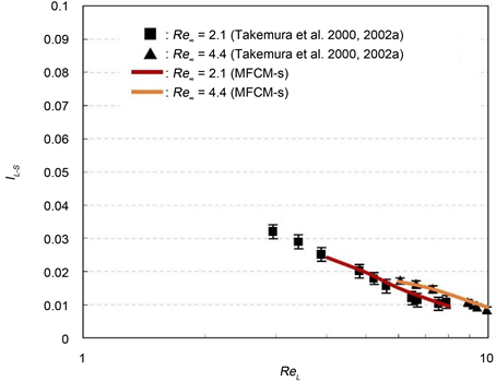
Figure 8. for and 4.4 as a function of by MFCM-s.

Figure 9. for , 7.3 and 15 as a function of by MFCM-s.
The second method is called MFCM-n, where FMT was modified according to the drag force equation given in [18] . This method was successfully applied to obtain the values of the lift force on a no-slip bubble for . The results agreed with those found by RFCM.
The third method is called MFCM-s, where FMT was modified according to the drag force equation given in [19] for a slip bubble. This method was successfully applied to obtain the values of the lift force on a slip bubble for . However, calculation results using RFCM for a slip bubble could not reproduce the experimental data.
In the present paper, it is found that the three newly proposed methods can correctly trace the trajectory of a bubble near a vertical wall for relatively large Reynolds numbers, regardless of whether the bubble has a slip or no-slip surface. In future study, we investigate the effects of the value of the Gaussian distribution’s width, , in FMT and the modification of in FDT and develop simulation methods to deal with the fluid which includes many bubbles.
Acknowledgements
S. Yanase would like to give his cordial thanks to the Ministry of Education, Culture, Sports, Science and Technology for the financial support through the Grant-in-Aids for Scientific Research No. 15K05814 and 15H0419919.
Cite this paper
Guan, C., Yanase, S., Matsuura, K., Kouchi, T. and Nagata, Y. (2017) Application of the Modified Force-Coupling Method of Tracing the Trajectories of Spherical Bubbles with Solid-Like and Slip Surfaces. Open Journal of Fluid Dynamics, 7, 657-672. https://doi.org/10.4236/ojfd.2017.74043
References
- 1. Shatat, M.M.E., Yanase, S., Takami, T. and Hyakutake, T. (2009) Drag Reduction Effects of Micro-Bubbles in Straight and Helical Pipes. Journal of Fluid Science and Technology, 4, 156-167. https://doi.org/10.1299/jfst.4.156
- 2. Matsuura, K., Ogawa, S., Kasaki, S., Koyama, K., Kodama, M. and Yanase, S. (2015) Cleaning Polymer Ink from a Glass Substrate Using Microbubbles Generated by Hydrogen Bubble Method. Separation and Purification Technology, 142, 242-250. https://doi.org/10.1016/j.seppur.2015.01.009
- 3. Hirt, C.W. and Nichols, B.D. (1981) Volume of Fluid (VOF) Method for the Dynamics of Free Boundaries. Journal of Computational Physics, 39, 201-225. https://doi.org/10.1016/0021-9991(81)90145-5
- 4. Cundall, P.A. and Strack, O.D.L. (1979) A Discrete Numerical Model for Granular Assemblies. Géotechnique, 29, 47-65. https://doi.org/10.1680/geot.1979.29.1.47
- 5. Peskin, C.S. (1972) Flow Patterns around Heart Valves: A Digital Computer Method for Solving the Equations of Motion. PhD Thesis, Albert Einstein College of Medicine, Yeshiva University, New York. https://www.researchgate.net/publication/34137471_Flow_patterns_around_heart_valves_a_digital_computer_method_for_solving_the_equations_of_motion
- 6. Fuchimoto, T., Yanase, S., Mizushima, J. and Senda, J. (2009) Dynamics of Vortex Rings in the Spray from a Swirl Injector. Fluid Dynamics Research, 41, Article ID: 045503. https://doi.org/10.1088/0169-5983/41/4/045503
- 7. Kempe, T. and Fröhlich, J. (2012) An Improved Immersed Boundary Method with Direct Forcing for the Simulation of Particle Laden Flows. Journal of Computational Physics, 231, 3663-3684. https://doi.org/10.1016/j.jcp.2012.01.021
- 8. Maxey, M.R. and Patel, B.K. (2001) Localized Force Representations for Particles Sedimenting in Stokes Flow. International Journal of Multiphase Flow, 27, 1603-1626. https://doi.org/10.1016/S0301-9322(01)00014-3
- 9. Xu, J., Maxey, M.R. and Karniadakis, G.E. (2002) Numerical Simulation of Turbulent Drag Reduction Using Micro-Bubbles. Journal of Fluid Mechanics, 468, 271-281. https://doi.org/10.1017/S0022112002001659
- 10. Takemura, F., Takagi, S. and Matsumoto, Y. (2000) Lift Force on a Spherical Gas Bubble Rising near a Plane Wall. Transactions of the Japan Society of Mechanical Engineers, Series B, 66, 2320-2326. (In Japanese) https://doi.org/10.1299/kikaib.66.649_2320
- 11. Takemura, F., Takagi, S., Magnaudet, J. and Matsumoto, Y. (2002) Drag and Lift Forces on a Bubble Rising near a Vertical Wall in a Viscous Liquid. Journal of Fluid Mechanics, 461, 277-300. https://doi.org/10.1017/S0022112002008388
- 12. Vasseur, P. and Cox, R.G. (1977) The Lateral Migration of Spherical Particle Sedimenting in Stagnant Bounded Fluid. Journal of Fluid Mechanics, 80, 561-591. https://doi.org/10.1017/S0022112077001840
- 13. Takemura, F., Takagi, S. and Matsumoto, Y. (2002) Lift Force on a Bubble Rising near a Wall in Water below Reynolds Number of 20. Transactions of the Japan Society of Mechanical Engineers, Series B, 68, 1684-1690. (In Japanese) https://doi.org/10.1299/kikaib.68.1684
- 14. Frumkin, A. and Levich, V. (1947) On Surfactants and Interfacial Motion. Zhurnal Fizicheskoi Khimii, 21, 1183.
- 15. Lomholt, S., Stenum, B. and Maxey, M. R. (2002) Experimental Verification of the Force Coupling Method for Particulate Flows. International Journal of Multiphase Flow, 28, 225-246. https://doi.org/10.1016/S0301-9322(01)00045-3
- 16. Dance, S.L. and Maxey, M.R. (2003) Incorporation of Lubrication Effects into the Force-Coupling Method for Particulate Two-Phase Flow. Journal of Computational Physics, 189, 212-238. https://doi.org/10.1016/S0021-9991(03)00209-2
- 17. Yeo, K. and Maxey, M.R. (2010) Simulation of Concentrated Suspensions Using the Force-Coupling Method. Journal of Computational Physics, 229, 2401-2421. https://doi.org/10.1016/j.jcp.2009.11.041
- 18. Clift, R., Grace, J.R. and Weber, M.E. (1978) Bubbles, Drops and Particles. Academic Press, New York.
- 19. Mei, R., Klausner, J.F. and Lawrence, C.J. (1994) A Note on the History Force on Spherical Bubble at Finite Reynolds Number. Physics of Fluids, 6, 418-420. https://doi.org/10.1063/1.868039
- 20. Guan, C., Yanase, S., Matsuura, K., Kouchi, T. and Nagata, Y. (2017) Numerical Study on Motion of a Spherical Bubble near Vertical Wall Using Modified Force-Coupling Method. Submitted to Nagare. (In Japanese)