Open Journal of Statistics
Vol.2 No.5(2012), Article ID:25839,10 pages DOI:10.4236/ojs.2012.25070
Data Fusion Using Empirical Likelihood
Department of Mathematics and Statistics, York University, Toronto, Canada
Email: stevenw@mathstat.yorku.ca
Received September 28, 2012; revised October 30, 2012; accepted November 15, 2012
Keywords: Data Fusion; Empirical Likelihood; Robust Estimation; Multiple Samples
ABSTRACT
The authors propose a robust semi-parametric empirical likelihood method to integrate all available information from multiple samples with a common center of measurements. Two different sets of estimating equations are used to improve the classical likelihood inference on the measurement center. The proposed method does not require the knowledge of the functional forms of the probability density functions of related populations. The advantages of the proposed method are demonstrated through extensive simulation studies by comparing the mean squared errors, coverage probabilities and average lengths of confidence intervals with those from the classical likelihood method. Simulation results suggest that our approach provides more informative and efficient inference than the conventional maximum likelihood estimator if certain structural relationship exists among the parameters of relevant samples.
1. Introduction
A common problem in clinical trials and other medical research is how to accurately and efficiently estimate parameters of interest when the current sample size is too small due to cost and time constraints. Usually there might exist certain surrogate populations with low sampling cost that could provide relevant information for the population of direct inferential interest. In this article, we propose a robust semi-parametric method to integrate related information from different sources to improve the classical likelihood method.
The classical likelihood approach is arguably the most widely used method in statistical inference. It has been routinely applied in almost all the statistical applications. Despite a great success and excellent asymptotic properties, the classical likelihood has known limitations associated with making inference for small sample sizes. Consider a thought experiment as follows. Suppose that a random experiment is to toss a coin twice. The parameter of interest, denoted as , is the probability of turning up head for this coin. The maximum likelihood estimator (MLE) of
  is denoted as
 . If the coin is a fair onethe MLE will obtain the following:
  and
and . Thus, the MLE would have 50% chance to make a nonsensical decision by using the MLE when the sample size is only two. In addition, suppose that for some reason we cannot use this coin any more but we can flip another coin instead. In this situation, the classical likelihood approach would not consider the second experiment since it comes from a different population unless a functional relationship between the two parameters is known. If the second population is related to the first one due to some connection between these two parameters, one should be able to utilize this connection and make better statistical inference.
Different statistical methodologies have been proposed in the literature to integrate information from different sources (or populations) in a very general setting, see [1] and [2], and referees therein. Most of these methods, however, face the challenge of accurately validating or evaluating the relevance of all related information to guard against the possibility of introducing a significant bias or contaminating the current sample. In other words, the magnitude of integration must be controlled carefully and in addition likelihood weights must be chosen judiciously in order to achieve any desired improvement in statistical inference. We propose to tackle this difficult problem using a robust semi-parametric empirical likelihood method to achieve more accurate and robust inferential results.
Empirical likelihood, which was first introduced in [3], is a nonparametric method of inference based on a datadriven likelihood ratio function. It allows the statistician to employ likelihood methods, without specifying a parametric model for the data. It enjoys both the flexibility of nonparametric methods and the efficiency of parametric likelihood. As shown in [4], empirical likelihood is a prominent efficient tool in estimating parameters by incorporating estimating equations into constrained maximization of the empirical likelihood function. In the problem we consider, the relevant information from different sources could be used by incorporating extra set of estimating equations in the empirical likelihood framework.
To obtain robust estimates, we use median as an estimate of center instead of mean. We propose here using two different kinds of estimating equations; one uses median and the other one uses a smoothed version of median. The smoothing technique is the one proposed in [5] to improve the coverage accuracy. Our method can be easily generalized to multiple samples with relevant information. Without loss of generality, we consider data with two populations in the sequel.
The rest of the paper is organized as follows. The methodology framework, the proposed empirical likelihood approach, and its theoretical properties are presented in Section 2. Results of simulation studies demonstrating the empirical performance are provided in Section 3. Conclusion and some discussion are provided in Section 4.
2. Methodology
Suppose there are two groups of data from different population but sharing the same parameter of interest. Assume that
 .
.
The second group of data  might be different from the first population, and

Our goal is to estimate ![]() by using both samples. Directly using the log-likelihood
by using both samples. Directly using the log-likelihood

we might get a biased estimation due to the difference between the two populations.
We propose a semi-parametric empirical likelihood method which only requires the independence of these two samples. To combine the second sample with the first one, we use the following semi-parametric empirical likelihood

where

and  is an estimating function. From the empirical likelihood theory, we know
  is maximized by
 , where
 ![]() is the Lagrange multiplier. We can rewrite the log likelihood function as
is the Lagrange multiplier. We can rewrite the log likelihood function as
 (1)
(1)
and

We call ![]() the robust semi-parametric empirical likelihood estimate (RSPELE).
the robust semi-parametric empirical likelihood estimate (RSPELE).
The advantage of the log profile likelihood function is that it does not depend on the likelihood weights which could be difficult to choose. In our propose method, we do not require that the probability density function of the second population is identical to the first population. By using the empirical likelihood method, we do not even need to specify the functional form of the underlying distribution of the second population. Therefore, we can gain robust estimates in the sense that model mis-specification problem is avoided. Consequently, our method can be employed in a relatively wide range of applications when the functional form of the probability density function is not known.
In the following, the theoretical properties of the proposed RSPELE estimator will be presented. For clarity, all proofs are postponed to the Appendix. Theorem 1 below shows that under some regularity conditions, the RSPELE estimator ![]() is consistent to
is consistent to .
.
Theorem 1 Let  be i.i.d. from
  and
and  be i.i.d. from an unknown distribution. Assume that
  satisfies the regularity conditions given in Shao (2003) on the normality of the maximum likelihood estimator in parametric models. Let
  be the true parameter. We further assume that A1) There exists a matrix
  such that

as .
.
A2)  exists when
  is sufficiently small and is continuous at
 .
.
A3) .
.
Then, it follows that  in probability in the neighborhood of
  such that
 .
.
The asymptotic distribution of the ![]() and
and ![]() is shown in Theorem 2.
is shown in Theorem 2.
Theorem 2 In addition to the conditions of Theorem 1we assume that , where b is a constant. We also assume that
  exists with probability one and the set of its discontinuity points has zero probability. Then

where
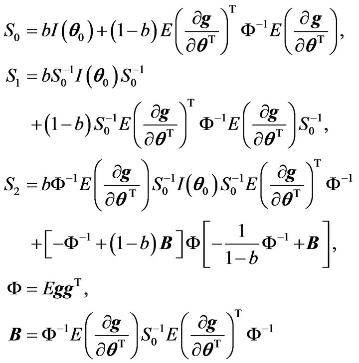 (2)
(2)
and  is the Fisher information about
  contained in X.
The asymptotic distribution of  is given in Theorem 3.
Theorem 3 Assume that the assumptions made in Theorem 2 hold. The limiting distribution of  is the same as the distribution of

under , where
  is independent of
 ,
,

and

where .
.
We note that other test statistics, for example, a test statistic based on Theorem 2, may also be used.
Estimating equations provide a very flexible way to specify how the parameters of a statistical model should be estimated. They serve as constraints in maximizing the empirical likelihood. It was shown in [5] that the empirical likelihood method is an efficient tool for point estimation through estimating equations. In this section, we consider two different kinds of estimating equations using the information of median, since median is robust with respect to the outliers, one may use

as estimating function based on the second group data, where  is the median of
  and
and  is the usual indicator function. It is easy to verify that
 .
.
Due to the discontinuity of , we may use the smoothed version of the constraint which was motivated by Shi and Lau (1999). First of all, we define the estimating equation for the smoothed empirical likelihood. In general, let
 ![]() be the
be the  -order kernel (Shi and Lau, 1999), such that

where r is a positive integer. Define
 For any
 , let
, let
 where h is called the smoothing parameter. The kernel
 ![]() is a symmetric probability density with bounded and compact support. Let the estimating function
is a symmetric probability density with bounded and compact support. Let the estimating function . Therefore,
  is continuous with respect to y, but it is not a fixed function as the smoothing parameter varies. See Shi and Lau (1999) for details. In addition, by using the arguments similar to those stated in the Theorems 1-3 and Shi and Lau (1999), we may get the similar asymptotic results.
3. Numerical Experiments
3.1. Data Fusion with Conventional Empirical Likelihood
Simulation studies are carried out by performing data fusion when two samples are available. The first sample
 is generated from standard normal distribution and the second sample
  is generated from normal, double exponential, or t-distribution respectively. The sample size of first sample,
  , is 10 and for the second sample, the sample size,
  , varies from 10, 20 to 30.
First of all we use the median constraint, so the log likelihood function of the simulation model is

where  is the MLE variance,
 .
.
We present the mean square error (MSE) ratio of RSPELE to MLE based on 1000 replications in Table 1. The simulation results show that RSPELE performs well except in the situation when the second population is normally distributed with large variation as the first one. When the second sample size is increasing, the RSPELE becomes more accurate. Moreover, we have smaller MSE of RSPELE when the data of the second population is more concentrated around the center, for example, the double exponential distribution.
3.2. Smoothed Empirical Likelihood
In this section we demonstrate the smoothed version of the estimating equations. The kernel we chose is the same as the one used in [6],

The simulation model is identical to the first experiment. Four values of the smoothed parameter are used which are  to the power of −1, −3/4, −1/2 and −1/4. The log likelihood function of the simulation model is

where  is the MLE variance.
We provide the MSE ratio of RSPELE to MLE based on 1000 replications in Table 2. Results of the smoothed version are slightly better than the results of the median version, no matter which smoothing parameter is chosen. When the underlying distribution of the second population is not the same as the first population, the RSPELE

Table 1. MSE ratio of RSPELE to MLE based on 1000 replications.

Table 2. MSE Ratio of RSPELE to MLE with the smoothing parameter h = n2 to the power of −1, −3/4, −1/2 and −1/4.
estimate performs better than the MLE. When the sample size of the second population is increasing, the RSPELE estimate is more accurate.
3.3. Confidence Intervals
In this subsection, we construct the confidence interval for the median by bootstrapping. In this simulation study, the first sample X is generated from standard normal distribution and the second sample Y is generated from normal, double exponential, or t-distribution. The sample size of X is 10 and of Y varies from 10, 20, to 30. The size of the bootstrapped sample is 200 and the number of iterations is set to be 1000. First of all, we use the median estimating equation and record the coverage probabilities and the simulated average confidence interval lengths (AL) in Table 3 for nominal levels of 80, 90, 95, and 99 percent. The coverage probabilities and the AL of using the smoothed version of the estimating equation are recorded in Tables 4 and 5 with different smoothing parameters which are  to the power of –1 and –1/2. We report the results of MLE in Table 6. Since the results of MLE do not depend on the second population, we further compare the coverage probabilities and AL as in Tables 3-5 with Table 6.
The results of smoothed version are better than median version in terms of the coverage probabilities. The coverage probabilities of RSPELE and MLE are very close but the confidence intervals of RSPELE are about 10% narrower than of MLE. The results of RSPELE when the underlying distribution of the second population is either t or double exponential distribution are better than the results of RSPELE when underlying distribution is normal distribution. That is because normal distribution is flatter than t and double exponential. Consequently, if the second population provides a good information about the center we can use it to get better estimates.

Table 3. Coverage probability of RSPELE with different distributions of second population by using median estimating equation, numbers show in the brackets are AL, α = nominal level.
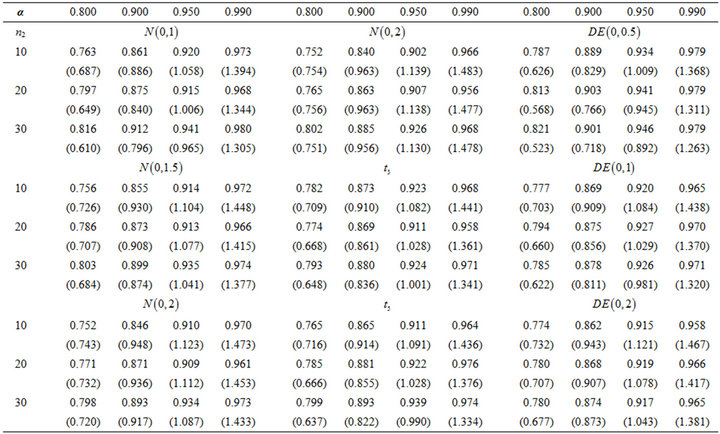
Table 4. Coverage probability of RSPELE with different distributions of second population, and the smoothing parameter , numbers show in the brackets are AL, α = nominal level.

Table 5. Coverage probability of RSPELE with different distributions of second population, and the smoothing parameter , numbers show in the brackets are AL, α = nominal level.

Table 6. Coverage probability of MLE with the distribution of second population normal, t3, t5 and double exponential, numbers show in the brackets are AL, α = nominal level.
4. Discussion
In this paper, we propose a robust semi-parametric empirical likelihood in a multiple-sample model with common measurement of center. We use two different kind of estimating equations of information about the median. Simulation studies have shown that the second population could provide very useful information on the parameter of interest by comparing the performance of various commonly used measures for evaluations.
5. Acknowledgements
We would like to thank Dr. Jing Qin for his generous and valuable comments and suggestions for this article.
REFERENCES
- X. Wang, C. van Eeden and J. V. Zidek, “Asymptotic Properties of Maximum Weighted Likelihood Estimators,” Journal of Statistical Planning and Inference, Vol. 119, No. 1, 2004, pp. 37-54.
- Y. Fu, X. Wang and C. Wu, “Weighted Empirical Likelihood Inference for Multiple Samples,” Journal of Statistical Planning and Inference, Vol. 139, No. 4, 2009, pp. 1462-1473.
- A. B. Owen, “Empirical Likelihood Ratio Confidence Interval for a Single Functional,” Biometrika, Vol. 75, No. 2, 1988, pp. 237-249.
- J. Qin and J. Lawless, “Empirical Likelihood and General Estimating Equations,” The Annals of Statistics, Vol. 22, No. 1, 1994, pp. 300-325.
- J. Shi and T. S. Lau, “Robust Empirical Likelihood for Linear Models under Median Constraints,” Communications in Statistics, Vol. 28, No. 10, 1999, pp. 2465-2479.
- J. Shao, “Mathematical Statistics,” Springer, New York, 2003. doi:10.1007/b97553
- A. B. Owen, “Empirical Likelihood,” Chapman & Hall/ CRC, New York, 2001. doi:10.1201/9781420036152
- Z. D. Bai, C. R. Rao and Y. Wu, “M-Estimation of Multivariate Linear Regression Parameters under a Covex Discrepancy Function,” Statistica Sinica, Vol. 2, 1992, pp. 237-254.
Appendix: Proofs
Proof of Theorem 1
We rewrite the Equation (1) as , where
  and
and
![]() . We denote
. We denote 
be the neighborhood of  such that
 ,
,  be the boundary of
 , i.e. for all
  such that
 be the neighborhood of
such that , and
, and .
.
Case 1. , where
 ![]() and
and  are two constants.
In view of the proof of Theorem 4.17 of [6], it follows that for any ,
,
 (3)
(3)
for large .
.
By Assumptions (A1)-(A3), applying a similar approach as in [7], it can be shown that . In light of the arguments in [4,8], and under the assumptions (A1)-(A3), it follows that for any
 ,
,
 (4)
(4)
for large .
.
Combining (3) with (4), we have for any ,
,

for large n. Therefore, there exists  such that
By the definition of , it follows that
  in probability.
Case 2. .
.
The consistency of ![]() can be shown similarly. The details are omitted.
can be shown similarly. The details are omitted. 
Proof of Theorem 2
We denote

Since

by applying Taylor’s expansion, it follows that

and

where . It is noted that

Hence we have

which can be written as

where

It can be shown that

Therefore, it follows that

where W is the covariance matrix of

with

 is independent of
  and
and

Since

with  and
and , it follows that

where


Proof of Theorem 3
Assume that the assumptions made in Theorem 3 hold. A statistic for testing  is given by
 (5)
(5)
Expending  around
  by Taylor’s expansion, we have
 (6)
(6)
Under , we have

which implies that

Hence,

(7)
Combining Equations (5)-(7), we have

Hence the limiting distribution of
 is the same as the distribution of
 under
under .
.