Journal of Modern Physics
Vol.3 No.2(2012), Article ID:17700,8 pages DOI:10.4236/jmp.2012.32027
Time Dilation as Field
Warsaw, Poland
Email: piotr.ogonowski@piotrogonowski.pl
Received November 29, 2011; revised January 6, 2012; accepted January 21, 2012
Keywords: Relativity; Maxwell Equations; Dilation; Lagrangian Mechanics
ABSTRACT
It is proved, there is no aether and time-space is the only medium for electromagnetic wave. However, considering time-space as the medium we may expect, there should exist field equations, describing electromagnetic wave as disturbance in time-space structure propagating in the time-space. I derive such field equations and show that gravitational field as well as electromagnetic field may be considered through one phenomena-time dilation.
1. Introduction
One of the main problems of the contemporary theoretical physics is Quantum Gravity (Bertfried Fauser, Jürgen Tolksdorf, Eberhard Zeidler, [1]).
The motivation to create this paper is conviction, that reformulation of the concept of fields by emphasis on itsrelationship with time dilatation factor and time-space structure may support to efforts to field unification.
Searching for Higgs boson or considering possible alternatives to Standard Model we try to explain issues, sort of:
● The nature of the elementary particle rest mass
● The nature of the photon energy
● Photon’s behavior on Planck’s energy scales.
The aim of this paper is tosupport issues mentioned above, by redefining electromagnetic field equations and stress similarity to Schwarzschild solution, what may open new ways for the quest for quantum gravity and the unified field theory.
Almost a hundred years have passed since 1908 when Hermann Minkowski gave a four-dimensional formulation of special relativity according to which space and time are united into an inseparable four-dimensional entity— now called Minkowski space or simply spacetime—and macroscopic bodies are represented by four-dimensional worldtubes. But so far physicists have not addressed the question of the reality of these worldtubes and spacetime itself” (Vesselin Petkov, page 1, [2]).
In this paper I reformulate Schwarzschild and Minkowski metrics and explain these metrics as consequence of introduced electromagnetic field description.
In first section I recall that one may consider curved time-space as collection of locally flat parts of Riemannian manifolds with assigned stationary observers. These infinite small flat fragments of time-space, according to transformed Schwarzschild solution and Rindler’s transformation appears to be accelerated. This approach allows us to define important reference frame, that may be used farther.
In second section I use above approach and introduce some fields, that binds together time flow and motion in d’Alembertians. Derived wave equation express disturbance in time-space structure propagating in time-space that may be explained as light.
In this paper we also refer to Max Planck’s Natural Units introduced in 1899. Let us then denote following designnations:
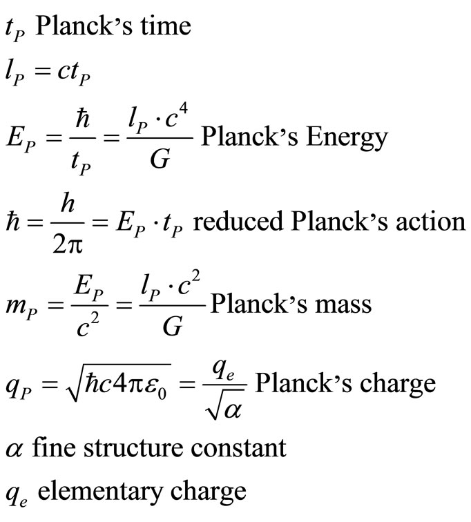 (1)
(1)
Farther I will deal with relativistic dynamics and show, that adding axis to Hamiltonian and Lagrangian we may obtain proper Lagrangian and Hamiltonian for gravitational field that one may understand as reformulation of the field interaction phenomena.
This way we develop farther the idea presented by Alexander Gersten: “(…) we have shown that thenon-relativistic formalism can be used provided the momenta and Hamiltonian belong to the same 4-vector.” (Alexander Gersten, page 10, [3]).
We will start with reference to the main equation of the General Theory of Relativity. We will narrow down our discussion to a spherically symmetrical mass to apply the Schwarzschild solution and then we will generalize above thanks to Rindler’s transformation.
2. Time Dilation as Field
2.1. Schwarzschild Metric and Time Dilation
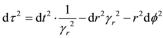
Let us start with recalling Schwarzschild metric (R. Aldrovandi and J. G. Pereira, page 111, [4]) and consider relation between gravitational potential and time dilation. To simplify calculations, in whole section we are assuming c = 1. For body orbiting at one plane around non-rotating big mass, we may write metric in form of:
 (2)
(2)
We assume:
●τ is the proper time of observer’s reference frame;
● t is the time coordinate (measured by a stationary clock at infinity);
● r is the radial coordinate;
● φ is the colatitude angle;
● vrs is the Schwarzschild radius.
According to this solution, the Schwarzschild’s radius and mass formulas are:
 (3)
(3)
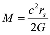 (4)
(4)
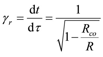
We introduce relativistic gamma factor:
 (5)
(5)
were call, that Schwarzschild’s solution drives to gravitational acceleration in “r” distance equal to:
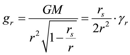 (6)
(6)
As we may easy calculate:
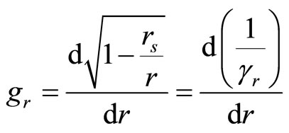 (7)
(7)
Above formula drives us to conclusion that relativistic gamma acts here as it would be scalar field. Let us explain above and its wide consequences in few steps.
At first step, let us rewrite Schwarzschild metric for some new reference frame. We start using formula (5):
 (8)
(8)
We may consider Schwarzschild metric for stationary observer, hanging at some point at distance “r” to source of gravitational force (such observer has to use some force to keep his position). We will denote such observer proper time as τobs:
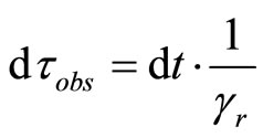 (9)
(9)
Now, we might rewrite Schwarzschild metric (8) referring to some local, chosen stationary observer reference frame and its proper time.
 (10)
(10)
If we will note above for geodesics we obtain:
 (11)
(11)
Above formula will be useful soon.
Using such stationary observer reference frame we recall that Riemannian manifolds are locally flat. If we shrink considered time-space into spheres with chosen “r” radius we obtain spherical, anisotropic Minkowski metric with slower coordinate light speed according to (11).
If we shrink it more, we consider infinitive small, local, part of chosen sphere, where photon meets Stationary Observer.
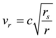
At second step, let us introduce velocity “vr”:
 (12)
(12)
We recognize velocity “vr” as Escape velocity and Free-falling velocity, thus we introduce some related spatial increment dxobs:
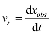 (13)
(13)
and then derive from (9) below formula:
 (14)
(14)
It is easy to notice, that above formula acts just like it would be Minkowski for free-falling velocity.
Now, at third step, let us recall Rindler’s transformation in some plane Minkowski time-spacefor body moving with acceleration “a”, achieving velocity “v”. We may consider such body using co-moving observer concept. We will denote its proper time as “τ” and note:
 (15)
(15)
 (16)
(16)
 (17)
(17)
Now, we may consider some hypothetical body with acceleration “gr”, achieving velocity “vr” with proper time “τr”.
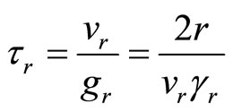 (18)
(18)
Let us perform following transformation:
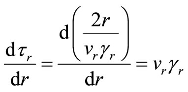 (19)
(19)
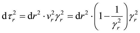 (20)
(20)
 (21)
(21)
Let us also introduce spatial increment as it would be inplane Minkowski metric. We will note this increment in polar coordinates:
 (22)
(22)
Let us note Minkowski metric for co-moving body:
 (23)
(23)
At the end, by substituting (21) we obtain:
 (24)
(24)
 (25)
(25)
Comparing above to (11) we recognize geodesics in Schwarzschild metric. Thus we must conclude that our Rindler transformationmight be done for accelerated light… To support above claim we will show in next section that rest mass existence is not necessary to consider acceleration for light.
We may also easy transform (18) to form of:
 (26)
(26)
Joining above with (7) we may explain acceleration by:
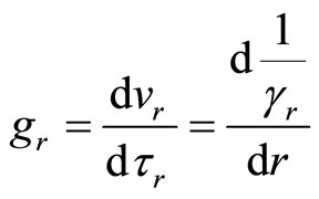 (27)
(27)
Gravitational acceleration gr may be then expressed by just introduced imaginary proper time τr and velocity vr.
Recalling (14) we should conclude, that geodesics in Schwarzschild metrics may be explained (besides classical explanation) as combination of two Minkowski metrics for:
(14) stationary observer moving against accelerated, freefalling surroundings (light)(11) free-falling surroundings (light) considered in relation to stationary observer proper time.
Referring to above conclusions we will introduce (in Section 3) reformulation of Lagrangian and Hamiltonian what might be understood as new description of field interactions.
2.2. Vector Fields for Minkowski Time-Space
As we know there is no ether and the medium for electromagnetic wave is time-space. We should expect, then, there must exists some field equations explaining electromagnetic wave as disturbance in time-space structure (structure of the medium) distributing in the time-space.
Let us prepare to such electromagnetic field description, describing at first some regular rotation of Planck’s mass mP, with line velocity vr, on the circle with radius R. We will define velocity as function of R equal to:
 (28)
(28)
where Rco is some defined constant.
Related gamma factor will be equal to:
 (29)
(29)
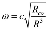
Angular velocity for rotating body we will denote as:
 (30)
(30)
Non-relativistic angular momentum we may denote as:
 (31)
(31)
 (32)
(32)
Non-relativistic radial acceleration we denote as:
 (33)
(33)
Maxwell has defined electromagnetic field phenomena by eliminating particles from equations while field sremains [5]. Let us do the same, but eliminating test body while motion and time flow remains.
We will construct vector fields to describe whole class of just introduced rotations defined for any place in space. Rest mass we may understand as parameter.
Let us define at first three versors nR, nx, ny. For any conductive vector R we define:
 (34)
(34)
 (35)
(35)
Let us define scalar field  and two related vector fields:
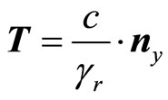 (36)
(36)
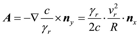 (37)
(37)
Please, note similarity of above A field to acceleration in Schwarzschild metric noted in (7) what will be useful soon. As we can easy show:
 (38)
(38)
 (39)
(39)
Let us define scalar field equal to  (related to angular momentum) and two auxiliary vector fields U and Ω.
 (40)
(40)
 (41)
(41)
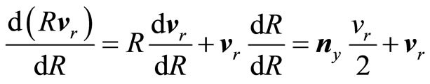
Let us notice, that:
 (42)
(42)
 (43)
(43)
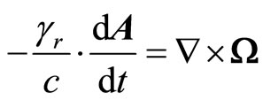
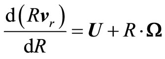
From above we derive:
 (44)
(44)
Let us also show, that:
 (45)
(45)
 (46)
(46)
Using (38) we obtain:
 (47)
(47)
From (44) and above we derive two d’Alembertians:
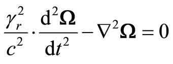 (48)
(48)
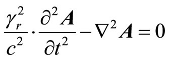 (49)
(49)
Above d’Alembertians describes wave with line velocity  or just time dilation around rotation center. Let us note the d’Alembertians in form of:
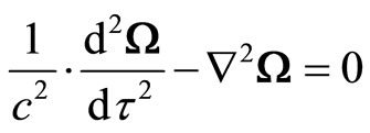 (50)
(50)
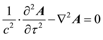 (51)
(51)
Above form of d’Alembertians describes move with “c” speed in infinite small, local part of time-space. This way in local reference frame light has always “c” speed.
We may also expect now, that derivative by R should act similar to derivative by proper-time. Let us perform some hypothetical calculation to prove it:
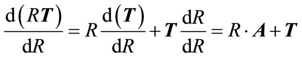 (52)
(52)
 (53)
(53)
 (54)
(54)
Now, let us analyze consequences of derived field equations and define Lagrangian and Hamiltonian for fields defined this way.
3. Reformulated Lagrangian and Hamiltonian
3.1. Lagrangian and Hamiltonian
Let us show how we may describe mechanics when we assign potential with gamma factor denoted as  and defined with formula (29).
Let us first recall a Hamiltonian expressed with general variables:
 (55)
(55)
where L is Lagrangian.
For three dimensional space we denote:
 (56)
(56)
Now, let us add extra zero-dimension and define velocity and momentum for such dimension. Let it be equal to defined previously rotation velocity (28) but here denoted with index “r” index:
 (57)
(57)
Summing expression for indexes 0 3 we define Hamiltonian in form of:
 (58)
(58)
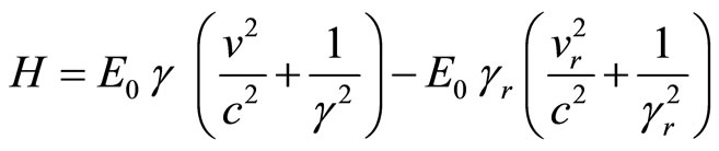
Now we define Lagrangian in form of:
 (59)
(59)
Thus:
 (60)
(60)
 (61)
(61)
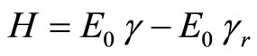 (62)
(62)
as we may easy see, in infinity above Hamiltonian express relativistic kinetic energy just as we should expect:
 (63)
(63)
as we will show in few steps, introduced Lagrangian and Hamiltonian drives to the same results then we may derive from GR for gravity.
3.2. Test for Lagrangian
Let us now check if introduced Lagrangian pass the tests.
At the beginning we should notice, that from (51) we obtain:
 (64)
(64)
Test condition for Lagrangian we should then rewrite as true only locally in form of:
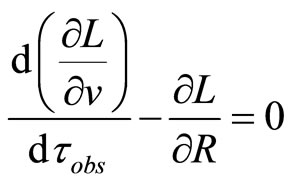 (65)
(65)
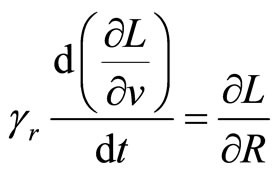 (66)
(66)
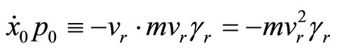
First derivative in LHS introduce momentum:
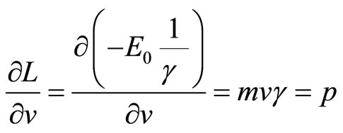 (67)
(67)
Next derivative result with relativistic force multiplied by gamma:
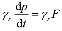 (68)
(68)
For RHS derivative drives to:
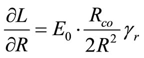 (69)
(69)
Let us compare (6) with obtained acceleration to notice, that we have obtained expected acceleration.
Substituting Schwarzschild radius in place of constant Rco and using (4) we could transform above to form of:
 (70)
(70)
We have obtained the force expected for introduced field. We will denote above force using “r” index:
 (71)
(71)
Now, using above and (68) we rewrite formula (66) as:
 (72)
(72)
As we may conclude, just derived relativistic force acting on body in every particular place in space is equal to force caused by field. Above is true for known fields.
3.3. Time-Space Curvature
Let us calculate divergence for line velocity:
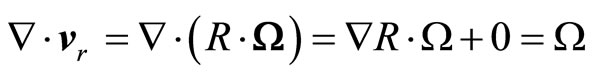 (73)
(73)
Now we calculate divergence for acceleration:
 (74)
(74)
 (75)
(75)
 (76)
(76)
Now we multiply and divide RHS by constants:
 (77)
(77)
Substituting Schwarzschild radius in place of constant Rco and using (4) we could transform above to form of:
 (78)
(78)
Let us denote mass density as:
 (79)
(79)
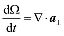
Let us express pulsation using rotating versor n. We obtain:
 (80)
(80)
 (81)
(81)
Using (51) we obtain:
 (82)
(82)
Now, using above to construct 4-dimentional conductive vector we obtain relation between mass density and time-space curvature the same as main equation of General Relativity.
3.4. Hamiltonian and Rest Energy Formula
Let us consider Hamiltonian for empty space. In place of test body’s rest energy let us use Planck’s Energy with meaning of unit “one”.
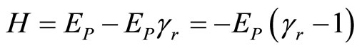 (83)
(83)
The smallest R we can substitute is Planck’s length.
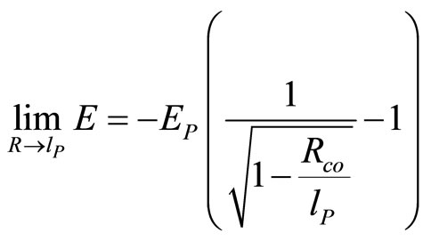 (84)
(84)
For very small constants we could rewrite equation using Maclaurin’s expansion:
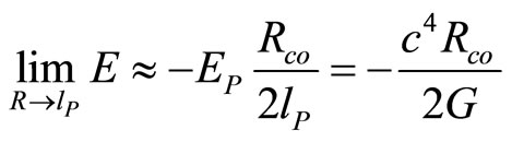 (85)
(85)
Let us notice similarity to rest energy formula, where Rco acts like Schwarzschild radius. We may conclude, that Schwarzschild radius might be explained as approximation of composition of set of some smaller particles with Rco  lP. Let us then define two variables for hypothetical mass and energy as follows:
 (86)
(86)
 (87)
(87)
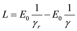
Now, we may easy show that introduced Hamiltonian approximates for small velocities and large distance Mechanical Energy defined by Newton. Let us transform (62) to form of:
 (88)
(88)
Using Maclaurin’s expansions of above for small velocities and large scales we obtain:
 (89)
(89)
 (90)
(90)
As we may see, above formula acts the same way that Newton’s Mechanical Energy formula.
4. Photon and Electrostatics Hypothesis
4.1. Photon Energy
Let us notice, that pulsation described in (30) is equal to:
 (91)
(91)
Non-relativistic angular momentum for such move is equal to:
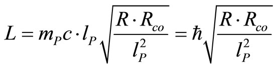 (92)
(92)
as we may notice, there is some Radius causing that angular momentum become equal to smallest action-reduced Planck’s action. Let us note such Radius with Rω and define as:
 (93)
(93)
Now we may introduce hypothetical gamma factor and rotation velocity with “E” index:
 (94)
(94)
 (95)
(95)
Kinetic Energy for such rotation is equal to:
 (96)
(96)
Now let us see, that  express pulsation in reference frame assigned to rotating frame. On a circle with radius R for line velocity
  we may note as follows:
 (97)
(97)
 (98)
(98)
Let then denote inverse of Radius as pulsation and write down:
 (99)
(99)
If we consider two twisted vectors of rotating field making double Helix, we will obtain well recognized formula:
 (100)
(100)
We may suppose that  describes electromagnetic field and the above quantum of energy may be assigned to photon. This way we may treat (50) and (51) as equivalent versions of Maxwell’s Equations [6].
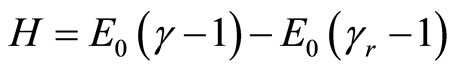
Pair production phenomena might be thus rewritten as:
 (101)
(101)
and after Maclaurin’s approximation:
 (102)
(102)
4.2. Electrostatics
The Electrostatic potential of two elementary charges, expressed in Planck’s units, can be noted as:
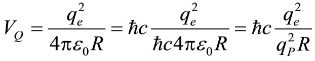 (103)
(103)
 (104)
(104)
Let us introduce auxiliary constant “ε” and variables:
 (105)
(105)
 (106)
(106)
We may understand above as equivalent of (85).
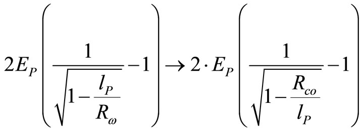
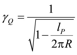
Now, let us assume that expression (104) is Maclaurin’s approximation for R  lP of interaction based on time dilation factor
 .
.
Therefore, it should follow below formula:
 (107)
(107)
as we can easy derive:
 (108)
(108)
 (109)
(109)
What astonishing, we have obtained epsilon close to 2π. It brings to mind De Broglie condition for length of the orbit. Let us follow this indication.
Let us redefine radius being limit for R in formula (106) using present knowledge. Now, we define auxiliary radius such way, to obtain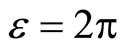 .
.
Let us introduce:
 (110)
(110)
 (111)
(111)
Let us redefine (106) and (107) as follows:
 (112)
(112)
 (113)
(113)
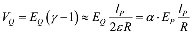
One may easy derive, that electrostatic force for two elementary charges may be expressed as:
 (114)
(114)
5. Summary
As we have just shown, the same field equations may describe as well electromagnetism as well gravity.
Field “A” defined in (37) may enter in place of:
● Electromagnetic field
● Gravitational acceleration.
Field “T” (36) and related scalar potential may act as:
● Electrostatic potential
●Gravitational potential.
Field “Ω” (41) may act as:
● Magnetic rotation
● Time-space curvature factor.
6. Acknowledgements
I would like to thank prof. Iwo Bialynicki-Birula from Polish Academy of Science for critique, asked me crucial questions and valuable time he had dedicated to me.
I would like to thank Dr. Rafal Suszek from Warsaw University for his time and lectures he has pointed to me.
I also thank to Dr. inz. Michal Wierzbicki from Warsaw University of Technology for his time and books he had borrowed to me.
I thank to Markus Nordberg from CERN for his interest and hints on early stage of the article.
I would like to thank posters from BAUT forum: caveman 1917, Celestial Mechanic, Kuroneko, Paul Logan, Tensor, Shaula, tusenfem, Garrison, macaw, grapes, slang, Strange, amazeofdeath, Geo Kaplan, pzkpfw, Eigen State, Jim, czeslaw, captain swoop, starcanuck 64 and Luckmeister. Thank you for your time, critique and questions. This article would never have matured without you. Especially I would like to thank to Celestial Mechanic for hope.
I dedicate this article to my Joanna, for the fact that I could work using the time, that should belong to her.
REFERENCES
- B. Fauser, J. Tolksdorf and E. Zeidler, “Quantum Gravity: Mathematical Models and Experimental Bounds,” Springer, Berlin, 2007.
- V. Petkov, “On the Reality of Minkowski Space,” Foundations of Physics, Vol. 37, No. 10, 2007, pp. 1499-1502. doi:10.1007/s10701-007-9178-9
- A. Gersten, “Tensor Lagrangians, Lagrangians Equivalent to the Hamilton-Jacobi Equation and Relativistic Dynamics,” Foundations of Physics, Vol. 41, No. 1, 2011, pp. 88-98. doi:10.1007/s10701-009-9352-3
- R. Aldrovandi and J. G. Pereira, “An Introduction to General Relativity,” Instituto de F´ısica Te´orica, Universidade Estadual Paulista, São Paulo, 2004.
- A. K. Prykarpatsky and N. N. Bogolubov Jr., “The Maxwell Electromagnetic Equations and the Lorentz Type Force Derivation—The Feynman Approach Legacy,” International Journal of Theoretic Physics, Vol. 51, No. 5, 2011, pp. 237-245.
- T. L. Gill and W. W. Zachary, “Two Mathematically Equivalent Versions of Maxwell’s Equations,” Foundations of Physics, Vol. 41, No. 1, 2011, pp. 99-128. doi:10.1007/s10701-009-9331-8