Positioning
Vol. 3 No. 2 (2012) , Article ID: 19589 , 8 pages DOI:10.4236/pos.2012.32003
Strapdown Navigation Using Geometric Algebra: Screw Blade Algorithm
![]()
Institute of Automation, National University of Defense Technology, Changsha, China.
Email: wudimin@nudt.edu.cn
Received February 8th, 2012; revised March 15th, 2012; accepted March 25th, 2012
Keywords: Inertial Navigation; Geometric Algebra; Screw Blade; Bortz Equation
ABSTRACT
The rigid body motion can be represented by a motor in geometric algebra, and the motor can be rewritten as a trinometric function of the screw blade. In this paper, a screw blade strapdown inertial navigation system (SDINS) algorithm is developed. The trigonometric function form of the motor is derived and utilized to deduce the Bortz equation of the screw blade. The screw blade SDINS algorithm is proposed by using the procedure similar to that of the conventional rotation vector attitude updating algorithm. The superiority of the screw blade algorithm over the conventional ones in precision is analyzed. Simulation results reveal that the screw blade algorithm is more suitable for the high-precision SDINS than the conventional ones.
1. Introduction
The strapdown inertial navigation system (SDINS) algorithm comprises attitude updating, velocity updating, and position updating, among which attitude updating usually utilizes the rotation vector algorithm [1-7]. The procedure of the rotation vector algorithm is: first, divide the attitude updating time interval equally into several segments and calculate the angular increment of each segment respectively; then, compute the total angular increment during the entire updating interval; finally, figure out the direction cosine matrix/quaternion of the updating time interval from the total angular increment. The theoretical foundation of the rotation vector algorithm is the Euler theorem, i.e., multiple rotations about axes passing through the origin is equivalent to a single rotation about some axis passing through the origin. Recently, a translation vector method, which is similar to the rotation vector algorithm, is proposed for the velocity/position updating [8].
According to the Chasles theorem, the rigid body motion can be represented by a rotation about an axis and a translation along that axis, and on this basis a SDINS algorithm based on dual quaternion (DQ) is presented [9]. The rotation vector and the translation vector are combined to construct the screw vector, which is utilized to calculate the DQs representing the vehicle’s motions. All navigation parameters can be extracted from these DQs. The velocity/position updating algorithms in both [8,9] are related to the rotation vector algorithm which has been commonly used in modern SDINS algorithms. However, the attitude updating is combined with the velocity and position updating in [9], which is different from in [8] or other references, where the attitude updating is generally manipulated separately from the velocity and position updating. The benefit of the DQ-based SDINS algorithm is that the structure of the navigation algorithm can be simplified, and the precision can be promoted.
Geometric algebra (GA), as well as DQ, is a unitary representational tool for the rigid body motion, but it is more general than the latter. Rotations and translations of any dimension can be depicted in GA.
Motivated by [9], recently we have proposed another SDINS model using GA [10]. The navigation equations were recast into three alike motor kinematic equations. As a test of the GA-based SDINS model, the fourth-order Runge-Kutta (RK) method was chosen to solve the motor kinematic equations. The results revealed that the precision of the RK-based SDINS algorithm was quite high. However, the RK method is computationally costly, and it requires a good smoothness of the integral function. To meet the real-time requirement and the unavoidable measurement error in the SDINS, this paper is about to develop a GA-based screw algorithm that is similar to the conventional rotation vector attitude updating algorithm.
The Contents of this paper are organized as follows. Section 2 reviews the GA SDINS model presented in [10]. Section 3 derives the trigonometric function form of the motor and the Bortz equation of the screw blade. A screw blade algorithm is developed in Section 4, and error analyses of the new algorithm and the conventional ones are presented in Section 5. In Section 6, a variety of simulations are carried out to testify the screw blade algorithm. Finally, concluding remarks are provided in Section 7.
2. Geometric Algebra Strapdown Inertial Navigation System Model
This section reviews the GA SDINS model, for detailed mathematical background please refer to [10] and references therein.
The purpose of inertial navigation is to provide navigation parameters through the integration of the angular rate and the total acceleration. The total acceleration consists of the specific force acceleration and the gravitational acceleration, which can be integrated into the thrust velocity and the gravitational velocity, respectively. Define the thrust velocity frame with its axes aligned with the body frame’s. The difference between the thrust velocity frame and the body frame is that the vector from the origin of the inertial frame to that of the thrust velocity frame is the thrust velocity, rather than the ordinary translation (See Figure 1). Similarly, we can define the gravitational velocity frame and the position frame. The axes of the gravitational velocity frame are aligned with those of the Earth-fixed frame. And the vector from the origin of the inertial frame to that of the gravitational velocity frame is the gravitational velocity. The position frame is attached to the centroid of the vehicle, and its axes are aligned with the Earth-fixed frame’s.
The kinematic equation of the motor that transforms the inertial frame  to the thrust velocity frame
  can be formulated as
 , (1)
, (1)
where
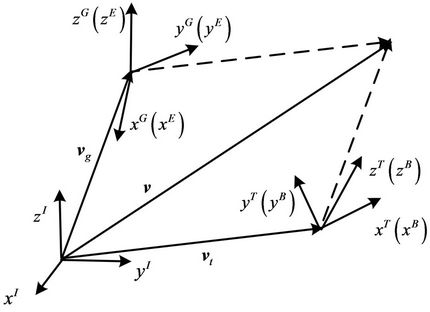
Figure 1. Velocity frames.
 , (2)
, (2)
in which  and
and  denote the angular rates of the thrust velocity frame
  and the body frame
  with respect to the inertial frame
 , respectively;
  denotes the thrust velocity;
  represents the rotor that transforms frame
  to frame
 ;
;  is the specific force acceleration; * is the dual operator; ~ is the reverse operator.
Similarly, the kinematic equation of the motor that transforms the inertial frame  to the gravitational velocity frame
  can be formulated as
 , (3)
, (3)
where
 , (4)
, (4)
in which  and
and  denote the angular rates of the gravitational velocity frame
  and the Earth-fixed frame
  with respect to the inertial frame
 , respectively;
  denotes the gravitational velocity;
  represents the rotor that transforms frame
  to frame
 ;
;  is the gravitational acceleration.
The kinematic equation of the motor that transforms the inertial frame  to the position frame
  can be formulated as
 , (5)
, (5)
where
 , (6)
, (6)
in which  denotes the angular rate of frame
  with respect to frame
 ;
;  denotes the position vector from the origin of frame
  to that of frame
 ;
;  represents the rotor that transforms frame
  to frame
 . The mechanism of the GA SDINS model is shown in Figure 2.
3. Screw Blade Bortz Equation
As shown in the last section, the kinematic equation of the motor has the unitary form
 , (7)
, (7)
where  denotes the screw velocity which consists of the angular rate
  and the velocity
 . It can be solved by traditional numerical integral algorithms. However, in order to meet the real-time requirements of the SDINS, a high-efficiency algorithm, which is similar to the rotation vector algorithm that has been widely used in the modern SDINS algorithm, needs to be developed. The rotation vector algorithm is based on the
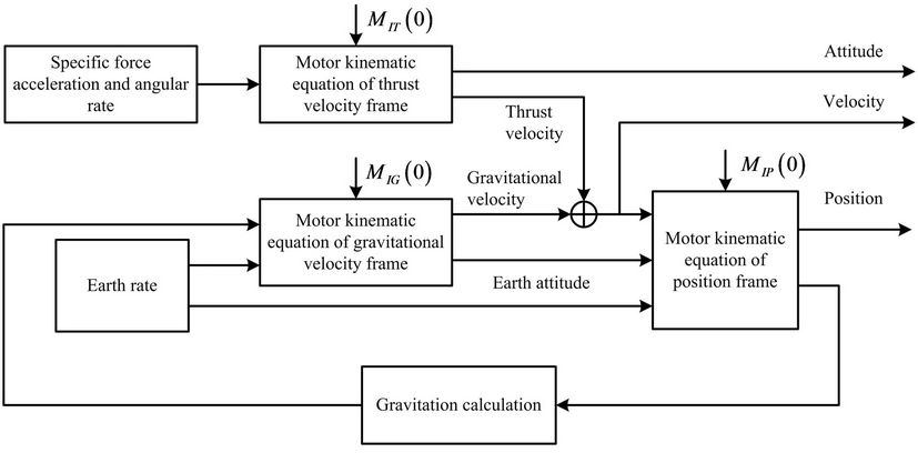
Figure 2. Mechanism of the GA SDINS model.
Bortz equation; therefore, we will build the GA-formed Bortz equation first.
A general rigid body motion can be constructed by a rotation in a plane around the origin, followed by a translation. As shown in Figure 3, the motor which represents the general rigid body motion, can be decomposed into the screw parameters as [11]
 , (8)
, (8)
where  and
and  represent the translation versor and the rotation versor (or rotor), respectively;
  represents the versor product;
 denotes the translation;
  denotes the plane in which the rotation is resident, and
 ;
;  is the rotation angle;
  is the translation along the rotation (or screw) axis;
  is the translation of the rotation axis.

Figure 3. Screw decomposition of the motor.
Define the screw blade to be , we have
 (9)
(9)
where  is the pseudoscalar;
  denotes the direction of the screw axis;
  denotes the magnitude of
 . It can be seen that
  is the right dual representation of the screw axis
 . Define
 , it can be shown that
 . (10)
Therefore, Equation (9) can be simplified as , or,
, or, . Considering that
  to the power of two or more equals zero, the motor can be rewritten as [12]
 (11)
(11)
where
 (12)
(12)
 . (13)
It is seen that the motor  is determined by the screw blade
 ; therefore,
  can be obtained if
  is known. Differentiating Equation (11) with respect to time gives
 . (14)
Substituting Equation (11) into the right side of Equation (7), yields
 (15)
(15)
where

is the cross product of two blades [11-13].
With Equations (7), (14), and (15), considering that terms of the same grade on one side of the equation should equal to those on the other side, it gives
 , (16)
 (17)
(17)
Substituting Equations (10) and (16) into Equation (17) gives
 . (18)
In fact, when  and
and , it follows that
 ,
,  ,
,  ,
, . (19)
Define , we have
 . (20)
Introducing Equations (19) and (20) into Equation (18), and multiplying the resultant equation with the pseudoscalar , Equation (18) can be simplified as
 , (21)
which is the Bortz equation of the rotation vector [1]. Therefore, Equation (18) can be considered as an extension of the Bortz equation, i.e., the Bortz equation of the screw blade.
4. Screw Blade Algorithm
Since the updating time interval is very short,  and
and  are small. Neglecting the second and higher orders of
  and
and , Equation (18) can be simplified as
 . (22)
Therefore, the screw blade increment of a time interval  can be computed as
 . (23)
in which  is the integral of the cross product, and it can be approximated as a noncommutative rate vector of the rotation vector [2,6]:
 , (24)
where
 .
.
On the other hand, the solution of Equation (22) in Taylor series is given by
 . (25)
Assume that the screw velocity can be represented by a third-order polynomial
 ,
,  , (26)
where  and
and  are constant blades. The 2-sample screw blade formula can be acquired by the following procedure:
1) Compute the differentiations of , and substitute them into Equation (25);
2) Divide the time interval evenly into 2 sub-intervals, and calculate the screw blade increment of each subinterval by integral of the screw velocity;
3) Compute the coefficients of the polynomial using the screw blade increments of the sub-intervals, and then substitute them into Equation (25).
It is found that
 , (27)
where  and
and  denote the screw blade increments of the sub-intervals. Other multiple samples screw blade formulae can be set up similarly. A general Nsample screw blade algorithm can be formulated as
 , (28)
where the constant coefficients  are the same as those in the rotation vector algorithms.
The motor of the updating interval can thus be calculated as
 , (29)
where . The total motor can be updated as
 , (30)
in which  and
and  represent the previous and current motors, respectively.
5. Algorithm Error Analysis
Since  is the integral of
 , we can assume
  , where
 ,
, . It follows that
 , (31)
where  is the magnitude of the rotation angleand
  is the magnitude of the translation along the screw axis. Therefore, Equation (11) can be expanded as
 (32)
(32)
On the other hand, the motor increment of the interval can be formulated as [11,12]
 . (33)
Therefore, the translation increment of the updating interval can be calculated as
 (34)
(34)
The relationship

is utilized in the above derivation.
Approximating the trigonometric functions by secondorder Taylor expansion, Equation (34) can be reduced to be
 . (35)
With Equations (22) and (28), the screw blade increment of the updating interval can be computed as
 (36)
(36)
where  is the screw blade increment of the sub-interval. Substituting (36) into (35) gives
 (37)
(37)
Its second-order approximation is
 . (38)
The last two terms in the above Equation are the sculling and rotation compensation terms in the conventional velocity integration [14,15]. Therefore, the error for the conventional algorithm includes: 1) approximation of the screw blade during the updating time interval in Equation (36); 2) truncation of trigonometric series to the second order in Equation (35); 3) approximation to second-order accuracy in Equation (38). On the other hand, the error for the screw blade algorithm comes from: 1) approximation of the screw blade in Equation (36); and 2) truncation of trigonometric functions in calculating Equation (34). Therefore, if the error in Equation (36) is small enough, the precision of the screw blade algorithm will be higher than that of the conventional ones. The error arisen from the approximation of the screw blade can be reduced by choosing high-precision inertial sensors to decrease measurement error, or by using big sample screw blade algorithms, or by shortening updating time intervals, etc.
6. Numerical Simulation
To testify the performance of the screw blade algorithm presented in this paper, a variety of experiments are carried out.
The navigation parameters and the gyro/accelerometer outputs are produced by an ideal trace generator. The inputs of the generator are the ground speed rate and the Euler angle rate, and the inputs for each channel are the same, which are  (m/s2) for the former, and
  (rad/s) for the latter. The frequencies are f = 0.01, 0.02, 0.04, 0.06, 0.08, 0.1, 0.2, 0.4, 0.6 and 0.8 (Hz). At the beginning, the vehicle stands still on the ground of the Earth at latitude 30˚ and longitude 110˚, and the attitude angles are all 0. The runtime is set to be 300 (s).
The coordinate transformation between the Earth fixed frame coordinate and the geodetic coordinate is achieved by an iterative algorithm proposed in [16]. To increase the precision, the gravitational acceleration is computed using the information of real time position of the vehicle. Since the position is calculated only once per updating interval, a third-order algorithm [17] is utilized in computing the screw blades of the gravitational velocity frame motor and the position frame motor.
In this test, the 2-sample screw blade algorithm is chosen to solve the GA SDINS model. For the conventional algorithm, 2-sample formulae are applied in attitude/velocity updating [4,18], and the trapezoidal integration is utilized in position updating.
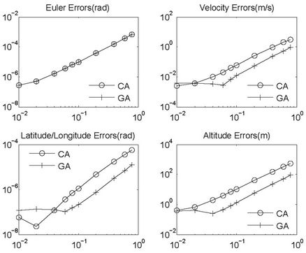
Here the measurement errors of the inertial sensors are simplified as a compound effect of the fixed bias and the Gaussian random noise. Four typical SDINS configurations used in the test are listed in Table 1. The maximum absolute errors (MAE) of both algorithms are illustrated in Figure 4 as a function of the varying input signal frequency. “CA” and “GA” stand for the conventional algorithm and the geometric algebra screw blade algorithm, respectively. The updating time interval is 0.02 (s).
It can be seen that:
1) The attitude errors of both algorithms are the same,
 (a)
(a)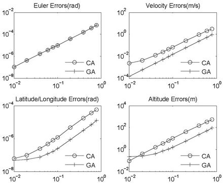 (b)
(b) (c)
(c) (d)
(d)
Figure 4. MAEs of algorithms with variant measurement errors as a function of varying input signal frequency. (a) Test 1; (b) Test 2; (c) Test 3; (d) Test 4.
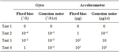
Table 1. Inertial sensor configuration.
but the velocity and position errors have been remarkably reduced due to the combination of the attitude updating and the velocity/position updating, which utilizes the highprecision attitude updating algorithm.
2) When there is no measurement error (Figure 4(a)), or the measurement error is minor (Figure 4(b)), the superiority of the GA over the CA is quite obvious. However, as the measurement error grows, the superiority loses gradually, as shown in Figure 4(d), in which the MAEs of both algorithms are almost the same. This is because the measurement error becomes the main error source of the algorithms as it grows.
3) There are some turning frequency points around which the MAEs of the CA are smaller than those of the GA. However, in most cases, the precision of the GA is better than that of the CA.
7. Conclusions
A screw blade algorithm is proposed to solve the GA SDINS model. At first, the trigonometric function form of the motor is derived by using the screw decomposition. The Bortz equation of the screw blade is deduced in succession. And then, the screw blade SDINS algorithm is developed similar to the conventional rotation vector attitude updating algorithm. The errors of the screw blade algorithm and the conventional ones are analyzed as well.
The performances of the screw blade algorithm are testified by a variety of simulations. The results reveal that the screw blade algorithm is a better choice than the conventional ones when the measurement error is small, and it is more suitable for the SDINS with high-precision requirement.
8. Acknowledgements
This project is supported by the National Natural Science Foundation of China (60835005). We appreciate Dr. Danfeng Zhou for his constructive suggestions in scientific writing.
REFERENCES
- J. E. Bortz, “A New Mathematical Formulation for Strapdown Inertial Navigation,” IEEE Transactions on Aerospace and Electronic Systems, Vol. AES-7, No. 1, 1971, pp. 61-66. doi:10.1109/TAES.1971.310252
- M. B. Ignagni, “Optimal Strapdown Attitude Integration Algorithms,” Journal of Guidance, Vol. 13, No. 2, 1990, pp. 363-369. doi:10.2514/3.20558
- M. B. Ignagni, “Efficient Class of Optimized Coning Compensation Algorithm,” Journal of Guidance, Control, and Dynamics, Vol. 19, No. 2, 1996, pp. 424-429. doi:10.2514/3.21635
- J. W. Jordan, “An Accurate Strapdown Direction Cosine Algorithm,” NASA TN-D-5384, 1969.
- J. G. Lee, Y. J. Yoon, J. G. Mark and D. A. Tazartes, “Extension of Strapdown Attitude Algorithm for High-Frequency Base Motion,” Journal of Guidance, Vol. 13, No. 4, 1990, pp. 738-743. doi:10.2514/3.25393
- R. B. Miller, “A New Strapdown Attitude Algorithm,” Journal of Guidance, Vol. 6, No. 4, 1983, pp. 287-291. doi:10.2514/3.19831
- P. G. Savage, “Strapdown Inertial Navigation Integration Algorithm Design Part 1: Attitude Algorithms,” Journal of Guidance, Control, and Dynamics, Vol. 21, No. 1, 1998, pp. 19-28. doi:10.2514/2.4228
- P. G. Savage, “A Unified Mathematical Framework for Strapdown Algorithm Design,” Journal of Guidance, Control, and Dynamics, Vol. 29, No. 2, 2006, pp. 237-249. doi:10.2514/1.17112
- Y. Wu, X. Hu, D. Hu, T. Li and J. Lian, “Strapdown Inertial Navigation System Algorithms Based on Dual Quaternion,” IEEE Transactions on Aerospace and Electronic Systems, Vol. 41, No. 1, 2005, pp. 110-132. doi:10.1109/TAES.2005.1413751
- D. Wu and Z. Wang, “Strapdown Inertial Navigation System Algorithm Based on Geometric Algebra,” Advances in Applied Clifford Algebras, Vol. 22, No. 1, 2012, pp. 1- 17.
- L. Dorst, D. Fontijne and S. Mann, “Geometric Algebra for Computer Science: An Object-Oriented Approach to Geometry,” 2nd Edition, Morgan Kaufmann Publishers, San Francisco, 2007.
- E. Bayro-Corrochano, “Geometric Computing for Wavelet Transforms, Robot Vision, Learning, Control and Action,” Springer Verlag, London, 2010.
- D. Hestenes, “New Foundations for Classical Mechanics,” 2nd Edition, Kluwer Academic Publishers, Dordrecht, 1999.
- M. B. Ignagni, “Duality of Optimal Strapdown Sculling and Coning Compensation Algorithms,” Journal of the Institute of Navigation, Vol. 45, No. 2, 1998, pp. 85-95.
- P. G. Savage, “Strapdown Inertial Navigation Integration Algorithm Design Part 2: Velocity and Position Algorithms,” Journal of Guidance, Control, and Dynamics, Vol. 21, No. 2, 1998, pp. 208-221. doi:10.2514/2.4242
- Y. Wu, P. Wang and X. Hu, “Algorithm of Earth-Centered Earth-Fixed Coordinates to Geodetic Coordinates,” IEEE Transaction on Aerospace and Electronic Systems, Vol. 39, No. 4, 2003, pp. 1457-1461. doi:10.1109/TAES.2003.1261144
- R. A. McKern, “A Study of Transformation Algorithms for Use in a Digital Computer,” M.S. Thesis, MIT, Cambridge, 1968.
- Y. Qin, “Inertial Navigation (in Chinese),” Science publisher, Beijing, 2006.