Dynamic Analysis for a SIQR Epidemic Model with Specific Nonlinear Incidence Rate

Jie Xu, Tiansi Zhang

College of Science, University of Shanghai for Science and Technology, Shanghai, China.

DOI: 10.4236/jamp.2019.78126                

Abstract

The article investigates a SIQR epidemic model with specific nonlinear incidence rate and stochastic model based on the former, respectively. For deterministic model, we study the existence and stability of the equilibrium points by controlling threshold parameter R₀ which determines whether the disease disappears or prevails. Then by using Routh-Hurwitz criteria and constructing suitable Lyapunov function, we get that the disease-free equilibrium is globally asymptotically stable if R₀<1 or unstable if R₀>1. In addition, the endemic equilibrium point is globally asymptotically stable in certain region when R₀>1. For the corresponding stochastic model, the existence and uniqueness of the global positive solution are discussed and some sufficient conditions for the extinction of the disease and the persistence in the mean are established by defining its related stochastic threshold R₀^s. Moreover, our analytical results show that the introduction of random fluctuations can suppress disease outbreak. And numerical simulations are used to confirm the theoretical results.

Keywords

Epidemic Model, Specific Nonlinear Incidence Rate, Lyapunov Function, Stability, Existence, Persistence

1. Introduction

Infectious diseases have always been a thorny issue that endangers human health, triggers social unrest and even affects national stability. Therefore, it is of great significance to take effective prevention measures to control the epidemic by establishing mathematical models with typical characteristics, discovering the transmission and development trends of infectious diseases. In the last decades, many authors have made a great headway on SIR (Susceptible-Infected-Removed) epidemic models [1] [2] [3] . However, for some diseases such as SARS, smallpox, foot-and-mouth disease, parrot fever and so on, introducing quarantine is one of the most pivotal and effective control means. In a model, assuming that some susceptible individuals become infected ones, and then the infected individuals flow into three parts, some remains at class I, some move into the removed R after recovering health, while some are transferred to the quarantine class Q and enter class R until they are no longer infectious. It is worth noting that the infected and quarantined people have permanent immunity after recovery. The model with the above characteristics is called SIQR (Susceptible-Infected-Quarantined-Removed) model. It is not difficult to find that a large amount of researches on the impact of quarantine on infectious diseases have been carried out so far [4] [5] [6] [7] . And in 2017, Joshi et al. [8] studied a SIQR epidemic model with saturated incidence rate and proved the global stability of the disease-free and endemic equilibrium.

In order to realistically reflect the process of human-to-human disease transmission, it is very important to determine the specific form of the incidence function which describes the increased number of infected people per unit time and plays a vital role in epidemiological dynamics research. Due to the complexity of disease transmission in real life, many scholars admit that the nonlinear incidence function is more reasonable than the bilinear incidence and standard incidence. The specific nonlinear incidence $\frac{\beta S\left(t\right)I\left(t\right)}{f\left(S\left(t\right)\mathrm{,}I\left(t\right)\right)}$ was proposed in 2013 [9] , where $f\left(S\left(t\right)\mathrm{,}I\left(t\right)\right)=1+{\alpha }_{1}S\left(t\right)+{\alpha }_{2}I\left(t\right)+{\alpha }_{3}S\left(t\right)I\left(t\right)$ and ${\alpha }_1\mathrm{,}{\alpha }_2\mathrm{,}{\alpha }_3$ are saturation factors that measure psychological or inhibitory effects and nonnegative constants. Obviously, depending on the values of ${\alpha }_1\mathrm{,}{\alpha }_2\mathrm{,}{\alpha }_3$, the incidence can be changed to various common types of incidence rates in existing literatures, including the bilinear incidence rate, the saturation incidence, Beddington-DeAngelis incidence [10] and Crowley-Martin response [11] . Therefore, it is more interesting and valuable than the saturation incidence and is also widely used to study epidemic diseases. For instance, Adnani et al. [12] introduced the effect of white noise into a SIRS epidemic model with the above incidence. They analyzed the global existence, positivity and boundedness of solutions, as well as the dynamics of stochastic model. And Hattaf et al. [13] applied the incidence to a stochastic delayed SIR epidemic model with temporary immunity. They proved that the model is mathematically and biologically well-posed and also obtained sufficient conditions for the extinction and persistence of the disease. However, there are few articles on the SIQR model with this incidence rate.

In this paper, to improve and generalize the model of Joshi et al. [8] , we propose a new SIQR epidemic model based on the incidence [9] . The deterministic differential equations of the model are as follows:

$\{\begin{array}{l}\frac{\text{d}S\left(t\right)}{\text{d}t}=A-\mu S\left(t\right)-\frac{\beta S\left(t\right)I\left(t\right)}{f\left(S\left(t\right)\mathrm{,}I\left(t\right)\right)},\\ \frac{\text{d}I\left(t\right)}{\text{d}t}=\frac{\beta S\left(t\right)I\left(t\right)}{f\left(S\left(t\right)\mathrm{,}I\left(t\right)\right)}-\left(\delta +\gamma +\mu +{\mu }_1\right)I\left(t\right),\\ \frac{\text{d}Q\left(t\right)}{\text{d}t}=\delta I\left(t\right)-\left(\rho +\mu +{\mu }_2\right)Q\left(t\right),\\ \frac{\text{d}R\left(t\right)}{\text{d}t}=\gamma I\left(t\right)+\rho Q\left(t\right)-\mu R\left(t\right).\end{array}$ (1)

The total population $N\left(t\right)$ is divided into four compartments and $N\left(t\right)=S\left(t\right)+I\left(t\right)+Q\left(t\right)+R\left(t\right)$, where $S\left(t\right)\mathrm{,}I\left(t\right)\mathrm{,}Q\left(t\right)$ and $R\left(t\right)$ are the number of the susceptible, infected, quarantined and recovered individuals at time t, respectively. The parameter constants have the following biological meanings: A is the recruitment rate of the susceptible through birth and immigration; $\mu$ is the natural death rate of the population; ${\mu }_1$ is the disease-caused mortality of infective individuals; ${\mu }_2$ is the disease-caused mortality of quarantined individuals; $\beta$ represents contact rate of an infected person with other compartment members per unit time; $\delta$ is the isolation rate of the compartment I quarantined directly to enter Q; $\gamma$ is the recovery rate of infected individuals; $\rho$ is the recovery rate of quarantined individuals. In addition, all parameters of model (1) are supposed to be nonnegative constants. Especially, A and $\mu$ are positive constants.

In fact, any system is more or less affected by environmental factors. Stochastic models can predict the future dynamics of the system accurately compared to their corresponding deterministic models. Therefore, when establishing population model, many stochastic biological systems and stochastic epidemic models have been presented and studied [14] [15] . One of the most main ways to introduce random effects is to directly perturb the parameters of the deterministic model by Gaussian white noise. As an expansion of model (1), now we introduce white noises into (1) by substituting the parameters ${\mu }_i\mathrm{,}\beta$ with ${\mu }_i+{\sigma }_i{B}_i\left(t\right)$ $\left(i=1,2\right)$ and $\beta +{\sigma }_3{B}_3\left(t\right)$, where $B\left(t\right)=\left(B_1\left(t\right),B_2\left(t\right),B_3\left(t\right)\right)$ is a standard Brownian motion. ${\sigma }_i^2>0$ $\left(i=1,2,3\right)$ denote the intensity of the white noise. Other parameters are the same as in model (1). Hence, the stochastic system is described by

$\{\begin{array}{l}\text{d}S\left(t\right)=\left(A-\mu S\left(t\right)-\frac{\beta S\left(t\right)I\left(t\right)}{f\left(S\left(t\right)\mathrm{,}I\left(t\right)\right)}\right)\text{d}t-\frac{{\sigma }_{3}S\left(t\right)I\left(t\right)}{f\left(S\left(t\right)\mathrm{,}I\left(t\right)\right)}\text{d}{B}_3\left(t\right),\\ \text{d}I\left(t\right)=\left(\frac{\beta S\left(t\right)I\left(t\right)}{f\left(S\left(t\right)\mathrm{,}I\left(t\right)\right)}-\left(\delta +\gamma +\mu +{\mu }_1\right)I\left(t\right)\right)\text{d}t-{\sigma }_{1}I\left(t\right)\text{d}{B}_1\left(t\right)\\ +\frac{{\sigma }_{3}S\left(t\right)I\left(t\right)}{f\left(S\left(t\right)\mathrm{,}I\left(t\right)\right)}\text{d}{B}_3\left(t\right),\\ \text{d}Q\left(t\right)=\left(\delta I\left(t\right)-\left(\rho +\mu +{\mu }_2\right)Q\left(t\right)\right)\text{d}t-{\sigma }_{2}Q\left(t\right)\text{d}{B}_2\left(t\right),\\ \text{d}R\left(t\right)=\left(\gamma I\left(t\right)+\rho Q\left(t\right)-\mu R\left(t\right)\right)\text{d}t.\end{array}$ (2)

This paper is organized as follows. In Section 2, we present some preliminaries which will be used in our following analysis. In Section 3, the existence and stability of the equilibrium points of deterministic system is analyzed. In Section 4, we study dynamics of the stochastic model. Firstly, the existence and uniqueness of the global positive solution is proved. Then, the extinction and persistence of the disease under certain conditions is discussed. Finally, numerical simulations are presented to illustrate our main results. Section 5 just provides a brief discussion and the summary.

2. Preliminaries

In this section, some notations, definitions and lemmas are provided to prove our main results. Let $\left(\Omega \mathrm{,}\mathcal{F}\mathrm{,}\mathbb{P}\right)$ be a complete probability space with a filtration ${\left\{{\mathcal{F}}_t\right\}}_{t\ge 0}$ satisfying the usual conditions (i.e. it is increasing and right continuous while ${\mathcal{F}}_0$ contains all $\mathbb{P}$ -null sets). And $B_i\left(t\right)\left(i=1,2,3\right)$ are defined on this complete probability space.

Consider the 4-dimensional stochastic differential equation

$\text{d}x\left(t\right)=f\left(x\left(t\right)\mathrm{,}t\right)\text{d}t+g\left(x\left(t\right)\mathrm{,}t\right)\text{d}B\left(t\right)\text{for}t\ge t_0\mathrm{,}$ (3)

with initial value $x_0\in {ℝ}_{+}^4$. We define the differential operator L of Equation (3) as follows:

$L=\frac{\partial }{\partial t}+{\displaystyle \underset{i=1}{\overset{4}{\sum }}}{f}_i\left(x,t\right)\frac{\partial }{\partial x_i}+\frac{1}{2}{\displaystyle \underset{i,j=1}{\overset{4}{\sum }}}{\left[g^{\text{T}}\left(x,t\right)g\left(x,t\right)\right]}_{ij}\frac{{\partial }^2}{\partial x_i\partial x_j}.$

Let L act on a nonnegative function $V\left(x\mathrm{,}t\right)\in {\mathcal{C}}^{\mathrm{2,1}}\left({ℝ}_{+}^4\times \left[t_0\mathrm{,}\infty \right);{ℝ}_{+}\right)$. Then,

$LV\left(x,t\right)=V_t\left(x,t\right)+V_x\left(x,t\right)f\left(x,t\right)+\frac{1}{2}trace\left[g^{\text{T}}\left(x,t\right)V_{xx}\left(x,t\right)g\left(x,t\right)\right],$

where ${ℝ}_{+}^4=\left\{x_i>0,i=1,2,3,4\right\}$. By Itô’s formula, $\text{d}V\left(x,t\right)=LV\left(x,t\right)\text{d}t+V_x\left(x,t\right)g\left(x,t\right)\text{d}B\left(t\right)$. For an integrable function $\chi$ on $\left[\mathrm{0,}+\infty \right)$, we define

$\langle \chi \left(t\right)\rangle =\frac{1}{t}{\displaystyle {\int }_0^t\chi \left(s\right)\text{d}s}\mathrm{.}$

Definition 2.1 System (2) is said to be persistent in the mean if

$\underset{t\to \infty }{\lim \inf }\langle I\left(t\right)\rangle >0a.s\mathrm{..}$

Moreover, we need the following lemma (see Lemma 5.1 in [16] ).

Lemma 2.2. Let $g\in \mathcal{C}\left({ℝ}_{+}\times \Omega \mathrm{,}ℝ\right)$ and $G\in \mathcal{C}\left({ℝ}_{+}\times \Omega \mathrm{,}ℝ\right)$. If there exist two real numbers ${\lambda }_0\ge 0$ and $\lambda >0$ for all $t\ge 0$, such that

$\ln g\left(t\right)\ge {\lambda }_{0}t-\lambda {\displaystyle {\int }_0^{t}g\left(s\right)\text{d}s}+G\left(t\right)\text{and}\underset{t\to \infty }{\lim }\frac{G\left(t\right)}{t}=0a.s.,$

then

$\underset{t\to \infty }{\lim \inf }\langle g\left(t\right)\rangle \ge \frac{{\lambda }_0}{\lambda }a\mathrm{.}s\mathrm{..}$

Lemma 2.3. Consider the following two systems

$\frac{\text{d}x}{\text{d}t}=f\left(t,x\right),\frac{\text{d}y}{\text{d}t}=g\left(y\right),$

where $x\mathrm{,}y\in {ℝ}^n$, f and g are continuous, satisfy local Lipschitz conditions in any compact set $X\subset {ℝ}^n$, and $f\left(t\mathrm{,}x\right)\to g\left(x\right)$ as $t\to +\infty$, so that the second system is the limit system for the first system. Let $\Phi \left(t\mathrm{,}{t}_0\mathrm{,}{x}_0\right)$ and $\phi \left(t\mathrm{,}{t}_0\mathrm{,}{y}_0\right)$ be solutions of these systems, respectively. Suppose that $e\in X$ is a locally asymptotically stable equilibrium of the limit system and its attractive region is

$W\left(e\right)=\left\{y\in X|\phi \left(t,t_0,y\right)\to e,t\to +\infty \right\}.$

Let $W_{\Phi }$ be the omega limit set of $\Phi \left(t\mathrm{,}{t}_0\mathrm{,}{x}_0\right)$. If $W_{\Phi }\cap W\left(e\right)\ne \varnothing$, then ${\lim }_{t\to +\infty }\Phi \left(t\mathrm{,}{t}_0\mathrm{,}{x}_0\right)=e$.

3. Dynamics of the Deterministic SIQR Model

3.1. The Existence of Equilibrium Points

For a population dynamics system, studying its equilibrium points is the precondition for predicting the development trend of populations within the system.

Theorem 3.1 System (1) has two equilibrium points, $E_0=\left(\frac{A}{\mu },0,0,0\right)$ for all parameter values and $E^{*}=\left(S^{*},I^{*},Q^{*},R^{*}\right)$ for $R_0>1$, here $S^{\mathrm{<mo>\; *\; </mo>}}\in \left(\mathrm{0,}\frac{A}{\mu }\right)$, $I^{\mathrm{<mo>\; *\; </mo>}}\mathrm{,}{Q}^{\mathrm{<mo>\; *\; </mo>}}$ and $R^{*}>0$.

Proof. Summing up all the equations of model (1), we find the following differential equation: $\frac{\text{d}N}{\text{d}t}=A-\mu N-{\mu }_{1}I-{\mu }_{2}Q$. By comparison theorem, we obtain that the solutions of model (1) exist in the region defined by $\Gamma =\left\{\left(S,I,Q,R\right)\in {ℝ}_{+}^4:S+I+Q+R\le \frac{A}{\mu },S\ge 0,I\ge 0,Q\ge 0,R\ge 0\right\}$. To get the equilibrium points, we set the right-side of equations to be 0,

$\{\begin{array}{l}A-\mu S-\frac{\beta SI}{f\left(S,I\right)}=0,\\ \frac{\beta SI}{f\left(S,I\right)}-\left(\delta +\gamma +\mu +{\mu }_1\right)I=0,\\ \delta I-\left(\rho +\mu +{\mu }_2\right)Q=0,\\ \gamma I+\rho Q-\mu R=0,\end{array}$ (4)

which yields

$I=\frac{A-\mu S}{\delta +\gamma +\mu +{\mu }_1},Q=\frac{\delta }{\rho +\mu +{\mu }_2}I,R=\left(\frac{\gamma }{\mu }+\frac{\rho \delta }{\mu \left(\rho +\mu +{\mu }_2\right)}\right)I,$

$\frac{\beta S}{f\left(S,\frac{A-\mu S}{\delta +\gamma +\mu +{\mu }_1}\right)}=\delta +\gamma +\mu +{\mu }_1.$

If $I=0$, the model (1) has a disease-free equilibrium $E_0=\left(\frac{A}{\mu },0,0,0\right)$ for all parameter values. And we can get the basic reproduction number $R_0=\frac{\beta A}{\left(\mu +{\alpha }_{1}A\right)\left(\delta +\gamma +\mu +{\mu }_1\right)}$ by using next generation method. The value $R_0$ represents the average number of secondary infections when an infected person enters fully susceptible population. If $I\ne 0$, $I=\frac{A-\mu S}{\delta +\gamma +\mu +{\mu }_1}>0$ implies $S<\frac{A}{\mu }$. Hence, there is no positive equilibrium point if $S>\frac{A}{\mu }$. Now, we consider the function $g\left(S\right)$ defined on the interval $\left[\mathrm{0,}\frac{A}{\mu }\right]$, where

$\begin{array}{c}g\left(S\right)=\frac{\beta S}{f\left(S\mathrm{,}\frac{A-\mu S}{\delta +\gamma +\mu +{\mu }_1}\right)}-\left(\delta +\gamma +\mu +{\mu }_1\right)\\ \triangleq h\left(S\mathrm{,}I\right)-\left(\delta +\gamma +\mu +{\mu }_1\right)\mathrm{.}\end{array}$

Obviously, $g\left(0\right)=-\left(\delta +\gamma +\mu +{\mu }_1\right)<0$ and $g\left(\frac{A}{\mu }\right)=\frac{\beta A}{\mu +{\alpha }_{1}A}-\left(\delta +\gamma +\mu +{\mu }_1\right)=\left(\delta +\gamma +\mu +{\mu }_1\right)\left(R_0-1\right)>0$ when $R_0>1$. Simultaneously, differentiating the function g, we gain $g^{\prime }\left(S\right)=\frac{\partial h}{\partial S}-\frac{\mu }{\delta +\gamma +\mu +{\mu }_1}\frac{\partial h}{\partial I}>0$. Because $g\left(S\right)$ is monotonically increasing in the interval $\left[\mathrm{0,}\frac{A}{\mu }\right]$, $g\left(0\right)<0$ and $g\left(\frac{A}{\mu }\right)>0$, the equation $g\left(S\right)=0$ has only one positive root by the zero theorem. That is, there exists a unique endemic equilibrium $E^{*}=\left(S^{*},I^{*},Q^{*},R^{*}\right)$ with $S^{\mathrm{<mo>\; *\; </mo>}}\in \left(\mathrm{0,}\frac{A}{\mu }\right)$.

3.2. The Stability of Equilibrium Points

In the biological sense, we analyze the stability of the disease-free equilibrium point and the endemic equilibrium point.

Theorem 3.2. The disease-free equilibrium $E_0$ of system (1) is globally asymptotically stable if $R_0<1$ and unstable if $R_0>1$.

Proof. Consider the Jacobian matrix of system (1) at $E_0$

$J\left(E_0\right)=\left(\begin{array}{cccc}-\mu & -\frac{\beta A}{\mu +{\alpha }_{1}A}& 0& 0\\ 0& \frac{\beta A}{\mu +{\alpha }_{1}A}-\left(\delta +\gamma +\mu +{\mu }_1\right)& 0& 0\\ 0& \delta & -\left(\rho +\mu +{\mu }_2\right)& 0\\ 0& \gamma & \rho & -\mu \end{array}\right).$

The characteristic equation of system (1) at $E_0$ is

${\left(\lambda +\mu \right)}^2\left[\lambda +\left(\rho +\mu +{\mu }_2\right)\right]\left[\lambda -\frac{\beta A}{\mu +{\alpha }_{1}A}+\left(\delta +\gamma +\mu +{\mu }_1\right)\right]=0.$

Clearly, ${\lambda }_{1,2}=-\mu <0$, ${\lambda }_3=-\left(\rho +\mu +{\mu }_2\right)<0$ and the positive and negative of the fourth eigenvalue depends on $R_0$. That is, ${\lambda }_4=\frac{\beta A}{\mu +{\alpha }_{1}A}-\left(\delta +\gamma +\mu +{\mu }_1\right)=\left(\delta +\gamma +\mu +{\mu }_1\right)\left(R_0-1\right)<0$ when $R_0<1$, ${\lambda }_4>0$ when $R_0>1$. Hence the disease-free equilibrium $E_0$ is locally asymptotically stable if $R_0<1$ and unstable if $R_0>1$.

Then we prove the global stability of the system (1) at the equilibrium $E_0$ when $R_0<1$. Taking the Lyapunov function $W_1\left(t\right)=I\left(t\right)$ into consideration, we get

$\begin{array}{c}{\stackrel{\dot{}}{W}}_1=\left(\frac{\beta S}{f\left(S,I\right)}-\left(\delta +\gamma +\mu +{\mu }_1\right)\right)I\\ \le \left(\frac{\beta A}{\mu +{\alpha }_{1}A}-\left(\delta +\gamma +\mu +{\mu }_1\right)\right)I\\ =\left(\delta +\gamma +\mu +{\mu }_1\right)\left(R_0-1\right)I\le 0.\end{array}$

Thus if $R_0<1$, ${\stackrel{\dot{}}{W}}_1\le 0$. And ${\stackrel{\dot{}}{W}}_1=0$ if and only if $I=0$. In this case, $\frac{\text{d}S}{\text{d}t}=A-\mu S$ indicates $S\to \frac{A}{\mu }$ as $t\to \infty$. Similarly, $Q\to 0$ and $R\to 0$ as $t\to \infty$. So the largest positive invariant set in $\left\{\left(S,I,Q,R\right)\in \Gamma :{\stackrel{\dot{}}{W}}_1=0\right\}$ is the singleton $E_0$. By Liapunov-Lasalle theorem, $E_0=\left(\frac{A}{\mu },0,0,0\right)$ is globally asymptotically stable in $\Gamma$.

Theorem 3.3. If $R_0>1$, the endemic equilibrium point $E^{\mathrm{<mo>\; *\; </mo>}}$ of the system (1) is globally asymptotically stable in the region $\Omega =\Gamma -\left\{\left(S,I,Q,R\right)\in \Gamma :I=0\right\}$.

Proof. Consider the Jacobian matrix of system (1) at $E^{\mathrm{<mo>\; *\; </mo>}}$

$J\left(E^{*}\right)=\left(\begin{array}{cccc}-\mu -\frac{\beta I^{*}+{\alpha }_2\beta I^{*2}}{f^2\left(S^{*},I^{*}\right)}& -\frac{\beta S^{*}+{\alpha }_1\beta S^{*2}}{f^2\left(S^{*},I^{*}\right)}& 0& 0\\ \frac{\beta I^{*}+{\alpha }_2\beta I^{*2}}{f^2\left(S^{*},I^{*}\right)}& \frac{\beta S^{*}+{\alpha }_1\beta S^{*2}}{f^2\left(S^{*},I^{*}\right)}-\left(\delta +\gamma +\mu +{\mu }_1\right)& 0& 0\\ 0& \delta & -\left(\rho +\mu +{\mu }_2\right)& 0\\ 0& \gamma & \rho & -\mu \end{array}\right).$

Let $C_1=\frac{\beta I^{*}+{\alpha }_2\beta I^{*2}}{f^2\left(S^{*},I^{*}\right)}$ and $C_2=\frac{\beta S^{*}+{\alpha }_1\beta S^{*2}}{f^2\left(S^{*},I^{*}\right)}$, then

$J\left(E^{*}\right)=\left(\begin{array}{cccc}-\mu -C_1& -C_2& 0& 0\\ C_1& C_2-\left(\delta +\gamma +\mu +{\mu }_1\right)& 0& 0\\ 0& \delta & -\left(\rho +\mu +{\mu }_2\right)& 0\\ 0& \gamma & \rho & -\mu \end{array}\right).$

Therefore the characteristic equation of system (1) at $E^{\mathrm{<mo>\; *\; </mo>}}$ is

$\left(\lambda +\mu \right)\left[\lambda +\left(\rho +\mu +{\mu }_2\right)\right]\left\{\left(\lambda +\mu +C_1\right)\left[\lambda +\left(\delta +\gamma +\mu +{\mu }_1\right)-C_2\right]+C_1{C}_2\right\}=0.$

Obviously, ${\lambda }_1=-\mu <0$, ${\lambda }_2=-\left(\rho +\mu +{\mu }_2\right)<0$ and the other two eigenvalues are determined by the following quadratic equation

$\begin{array}{l}{\lambda }^2+\left[C_1+\mu +\left(\delta +\gamma +\mu +{\mu }_1\right)-C_2\right]\lambda \\ +\left(C_1+\mu \right)\left[\left(\delta +\gamma +\mu +{\mu }_1\right)-C_2\right]+C_1{C}_2=0\end{array}$

$\Rightarrow {\lambda }^2+a_1\lambda +a_2=0,$

where

$\begin{array}{l}{a}_1=C_1+\mu +\left[\left(\delta +\gamma +\mu +{\mu }_1\right)-C_2\right],\\ a_2=C_1\left(\delta +\gamma +\mu +{\mu }_1\right)+\mu \left[\left(\delta +\gamma +\mu +{\mu }_1\right)-C_2\right].\end{array}$

By utilizing Routh-Hurwitz criteria, we know that the system is stable if $a_1,a_2>0$ and unstable if $a_1,a_2<0$. From the second equation of (4), we obtain $\left(\delta +\gamma +\mu +{\mu }_1\right)>C_2$, thus all eigenvalues have negative real parts. The endemic equilibrium $E^{\mathrm{<mo>\; *\; </mo>}}$ is locally asymptotically stable.

Now we confirm the global stability at the equilibrium $E^{\mathrm{<mo>\; *\; </mo>}}$ when $R_0>1$. The first two equations of system (1) do not contain Q and R, so we consider the following Lyapunov function in the positive quadrant of the two-dimensional plane SI.

$W_2\left(t\right)=S-S^{*}-{\displaystyle {\int }_{S^{*}}^S}\frac{l\left(S^{*},I^{*}\right)}{l\left(x,I^{*}\right)}\text{d}x+I^{*}\Psi \left(\frac{I}{I^{*}}\right),$

where $l\left(S,I\right)=\frac{\beta S}{f\left(S,I\right)},\Psi \left(x\right)=x-1-\ln x,x>0$. Clearly,attains its global minimum at and. Besides, the function has the global minimum at and. Then,for any and for any. Consequently,with equality holding if and only if for all. And, So the derivative function of is given by

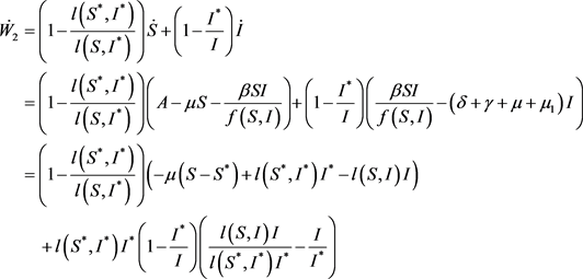
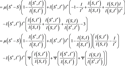
Due to

we have,, thus and if and only if and. By the Liapunov-Lasalle theorem, all solutions starting in the positive quadrant of SI-plane with approach at. In this case, the differential equation for Q has the limiting equation which implies as, and similarly, the limiting equation for R is so that as. Therefore, by Lemma 2.3, the endemic equilibrium is globally asymptotically stable in the region for the system (1). This completes the proof.

4. Dynamics of the Stochastic SIQR Model

4.1. Existence and Uniqueness of the Global Positive Solution

In order to study the dynamics of stochastic models, the primary question to be considered is whether the solution is global and nonnegative existence. Although the coefficients of the model (2) satisfy the local Lipschitz condition, it’s not enough to prove that the solution does not explode within a finite time for any given initial value. Hence in this section, we will show that the solution of model (2) is positive and global.

Theorem 4.1. For any given initial value

, there exists a unique solution of system (2) on, which is in with probability one.

Proof. Since the system (2) has locally Lipschitz continuous coefficients, then for any initial value, system (2) has a unique local solution on, where is the explosion time. To verify this solution is global, we only need to show that. Now define the stopping time as

Set (denotes the empty set). Obviously, if we can show, then. Assume that this statement is false, then there exists a constant such that.

Define a -function by

Applying Itô’s formula, for all, we obtain

where

Since for all, and, we have

Hence,

(5)

From the definition of, it follows that. Therefore,

Letting in (5) and then taking the expectation on both sides of (5), we have that

which is a contradiction and we confirmed. This completes the proof.

Remark 4.2. The region is almost surely positive invariant of stochastic model (2), refer to [12] . In addition, from biological consideration, we next focus on the disease dynamics of model (2) in the bounded set.

4.2. The Extinction and Persistent in the Mean of the Disease

One of the most concerning issues in epidemiology is how to establish the threshold condition for the extinction and persistence of the disease. The target of this section is to study the extinction and persistence of the disease. First of all, we define corresponding random threshold as follows:

Theorem 4.3. Let be a solution of system (2) for any given initial value.

1) If and, then

(6)

2) If, then

(7)

which means that tends to zero exponentially a.s., i.e. the disease dies out with probability 1. Furthermore,

(8)

Proof. Define Lyapunov function, by Itô’s formula, we get that

(9)

where.

Suppose 1) holds. Noting that is monotone increasing for and, we have

Then,

Integrating both sides of the above inequality from 0 to t and dividing by t, we obtain

(10)

where. By the strong law of large numbers for local martingales [17] , we derive that. Since, Equation (10) becomes

We obtain the desired assertion (6).

If 2) holds, from Equation (9), we get

(11)

Since, Equation (11) becomes

We obtain the desired assertion (7). And so

(12)

From the first two equations of system (2), there is

(13)

Integrating both sides of (13) from 0 to t and dividing by t, we have

Therefore,

(14)

where. Clearly,and from (12), we have

Therefore the assertion (8) holds. The conclusion is proven.

Next, the conditions for the persistence of the disease are presented.

Theorem 4.4. Suppose that, then the solution of system (2) is persistent in the mean for any given initial value. Moreover,

(15)

(16)

(17)

(18)

where

Proof. Since, we have

Then

(19)

Integrating both sides of (19) from 0 to t, there is

From (14), we have

where. Obviously,

. By Lemma 2.2 and, we deduce that

This is the required inequality (15), and from (14), we have

Therefore,

the inequality (16) is valid. From the third equation of system (2), we have

Then,

where. It follows from the strong law of large numbers for local martingales that, hence (17) holds for

The last equation of system (2) gives

Then,

So we have

This is the required inequality (18).

4.3. Numerical Simulations

In this section, we numerically simulate solutions of the models by using the Milstein’s method [18] to confirm main results. We compare the threshold parameters of the deterministic model and stochastic model to illustrate the effect of white noise on the system. The model (2) can be rewritten as the following discrete equation:

where and,are the Gaussian random variables. Similarly, the model (1) can also be written in the above form. We just need to delete the disturbance term and will not repeat it here.

Example 4.3.1 For the deterministic system (1), we choose the initial value and the parameter values,,,,,,,,,,. By Matlab software, we get and find that the class I, Q and R tend to 0, which means that the disease dies out (see Figure 1(a)). Theorem 3.2 is illustrated. Then, let and,,,,,,,,,,to draw Figure 1(b). It shows that the disease becomes endemic and. The condition of theorem 3.3 is satisfied.

Example 4.3.2 For the stochastic system (2), we choose the initial value and the parameter values,,,,,,,,,,,,,. By calculation,and. Hence, the condition 1) of theorem 4.3 is satisfied. In Figure 2(a), the class I exponentially decays to zero which indicates the extinction of the disease. Next, we let parameter and others are the same as above. In this case,. Therefore, the condition 2) of theorem 4.3 is satisfied and the disease dies out (Figure 2(b)). Finally, let,,,,and keep the other parameters, we get. According to theorem 4.4, all classes of the system (2) are persistent and are shown in Figure 2(c).

(a)(b)

Figure 1. Dynamics of the deterministic system (1).

(a)(b)(c)

Figure 2. Dynamics of the stochastic system (2).

Example 4.3.3 Now, we reselect the parameters ,,,,,,,,,,,,,,and give a set of comparison charts of simulation results. In Figure 3,, the class S, I, Q and R of deterministic model all exist, which means that the disease break out, but after adding white noise, except for the class S, the others tend to be 0. It reveals that the random fluctuations can suppress disease prevail.

5. Summary and Discussions

In this work, we investigate the deterministic and stochastic SIQR epidemic models with the specific nonlinear incidence. This incidence rate can become multiple types, and is more abundant than saturation incidence. We obtain the

(a)(b)(c)(d)

Figure 3. The random fluctuations can suppress disease break out.

dynamics properties of the SIQR model based on two threshold parameters and. And owing to, there may be an interesting situation, which indicates that the random fluctuations can suppress disease break out. Moreover, we simulate them with computer software and the results of the simulation are also consistent with the theoretical results. It can provide us with some useful control strategies to regulate disease dynamics.

In future work, we will further consider the delayed SIQR model with this incidence and the SIQS model without permanent immunity.

Conflicts of Interest

The authors declare no conflicts of interest regarding the publication of this paper.

References

[1]	Jiang, D.Q., Yu, J.J. and Ji, C.Y. (2011) Asymptotic Behavior of Global Positive Solution to a Stochastic SIR Model. Mathematical and Computer Modelling, 54, 221-232. https://doi.org/10.1016/j.mcm.2011.02.004
[2]	Hattaf, K., Lashari, A.A., Louartassi, Y. and Yousfi, N. (2013) A Delayed SIR Epidemic Model with General Incidence Rate. Electronic Journal of Qualitative Theory of Differential Equations, 3, 1-9. https://doi.org/10.14232/ejqtde.2013.1.3
[3]	Fan, K.G., Zhang, Y., Gao, S.J. and Wei, X. (2017) A Class of Stochastic Delayed SIR Epidemic Models with Generalized Nonlinear Incidence Rate and Temporary Immunity. Physica A: Statistical Mechanics and Its Applications, 481, 198-208. https://doi.org/10.1016/j.physa.2017.04.055
[4]	Alakes, M., Prosenjit, S. and Samanta, G.P. (2018) Analysis of an SIQR Model. Journal of Ultra Scientist of Physical Sciences, 30, 218-226. https://doi.org/10.22147/jusps-A/300307
[5]	Lan, G.J., Chen, Z.W., Wei, C.J. and Zhang, S.W. (2018) Stationary Distribution of a Stochastic SIQR Epidemic Model with Saturated Incidence and Degenerate Diffusion. Physica A: Statistical Mechanics and Its Applications, 511, 61-77. https://doi.org/10.1016/j.physa.2018.07.041
[6]	Chahrazed, L. and Lazhar, R.F. (2013) Stability of a Delayed SIQRS Model with Temporary Immunity. Advances in Pure Mathematics, 3, 240-245. https://doi.org/10.4236/apm.2013.32034
[7]	Zhang, X.B. and Huo, H.F. (2014) Dynamics of the Deterministic and Stochastic SIQS Epidemic Model with Nonlinear Incidence. Applied Mathematics and Computation, 243, 546-558. https://doi.org/10.1016/j.amc.2014.05.136
[8]	Joshi, H. and Sharma, R.K. (2017) Global of an SIQR Epidemic Model with Saturated Incidence Rate. Asian Journal of Mathematics and Computer Research, 21, 156-166.
[9]	Adnani, J., Hattaf, K. and Yousfi, N. (2013) Stability Analysis of a Stochastic SIR Epidemic Model with Specific Nonlinear Incidence Rate. International Journal of Stochastic Analysis, 2013, Article ID: 431257. https://doi.org/10.1155/2013/431257
[10]	Ji, C.Y. and Jiang, D.Q. (2011) Dynamics of a Stochastic Density Dependent Predator-Prey System with Beddington-DeAngelis Functional Response. Journal of Mathematical Analysis and Applications, 381, 441-453. https://doi.org/10.1016/j.jmaa.2011.02.037
[11]	Crowley, P.H. and Martin, E.K. (1989) Functional Responses and Interference within and between Year Classes of a Dragonfly Population. Freshwater Science, 8, 211-221. https://doi.org/10.2307/1467324
[12]	Adnani, J., Hattaf, K. and Yousfi, N. (2016) Analysis of a Stochastic SIRS Epidemic Model with Specific Functional Response. Applied Mathematical Sciences, 10, 301-314. https://doi.org/10.12988/ams.2016.511697
[13]	Hattaf, K., Mahrouf, K. and Adnani, J. (2018) Qualitative Analysis of a Stochastic Epidemic Model with Specific Functional Response and Temporary Immunity. Physica A: Statistical Mechanics and its Applications, 490, 591-600. https://doi.org/10.1016/j.physa.2017.08.043
[14]	Li, D., Cui, J.A., Liu, M. and Liu, S.Q. (2015) The Evolutionary Dynamics of Stochastic Epidemic Model with Nonlinear Incidence Rate. Bulletin of Mathematical Biology, 77, 1705-1743. https://doi.org/10.1007/s11538-015-0101-9
[15]	Cai, Y.L., Kang, Y. and Wang, W.M. (2017) A Stochastic SIRS Epidemic Model with Nonlinear Incidence Rate. Applied Mathematics and Computation, 305, 221-240. https://doi.org/10.1016/j.amc.2017.02.003
[16]	Ji, C.Y. and Jiang, D.Q. (2014) Threshold Behaviour of a Stochastic SIR Model. Applied Mathematical Modelling, 38, 5067-5079. https://doi.org/10.1016/j.apm.2014.03.037
[17]	Chang, Z.B., Meng, X.Z. and Lu, X. (2017) Analysis of a Novel Stochastic SIRS Epidemic Model with Two Different Saturated Incidence Rates. Physica A: Statistical Mechanics and Its Applications, 472, 103-116. https://doi.org/10.1016/j.physa.2017.01.015
[18]	Higham, D.J. (2001) An Algorithmic Introduction to Numerical Simulation of Stochastic Differential Equations. Society for Industrial and Applied Mathematics, 43, 525-546. https://doi.org/10.1137/S0036144500378302