1. Problem Statement
In recent years, climate change has evolved from being a mere scientific theory to a real phenomenon, which is receiving a lot of publicity in the media.
Increased emissions of anthropogenic greenhouse gases are leading to a dramatic change in the atmosphere [1] . These changes have a negative effect on the natural human environment. As a result, climate change is causing a considerable increase in extreme weather conditions, such as severe precipitation, flooding or heat waves [2] .
However, it is not just global climate change which is an imminent problem for mankind. When ecological conditions are altered by people, local climate will also be transformed. This local climate change is particularly pronounced in cities. This can, for example, lead to urban heat islands, which can amount to up to 10 K in large cities. In addition to this, there is also an extensive effect on local wind fields, air pollution control as well as on an urban water balance [3] . Urban vegetation is in constant interaction with the atmosphere. On the one hand, vegetation impacts the atmosphere through e.g. clouding and humidity effects. On the other hand, vegetation adapts to the altered boundary conditions by changing its growth cycles as well as the species composition [4] .
An area-wide confirmation of this urban climate effect is only possible through extensive and usually expensive empirical surveys or complex modelling [5] . For this reason, studies of the urban climate are mainly carried out in large cities. However, even in small settlements local climate can have a negative impact on humans [6] . In order to plan settlement developments which are suitable for urban climate, local conditions must first be analysed. Currently used methods cannot provide low-cost solutions which deliver sufficient findings with regards to how detailed and current the data are.
2. The Matrix Method
2.1. Introduction to the Matrix Method
The approach of gathering urban-climate-relevant indicators locally, even in small settlements, in order to identify possible problem areas, is already providing a starting point for ecological urban development. Many of these indicators only start showing an effect when used in combination with other indicators [7] . In order to record these interdependencies and to obtain detailed and robust primary data for suggested courses of action, two different indicators are evaluated and then illustrated in a matrix. This allows for individual sub-areas, which hold potential for a particular climatic phenomenon in settlements, to be easily and effectively visualized, and thus identified.
The matrices used for the evaluation of the urban ecology are in a simple table format. Thereby, the two indicators are divided into different categories. Next, the two indicators are arranged in the table in such a way so that the categories showing the best characteristics in terms of urban ecology will be found in the top left hand corner. Figure 1 shows a schematic representation of the resulting matrix. The concluding urban-ecological evaluation of each cell can be varied from matrix to matrix. This matrix method allows for various combinations of indicators.
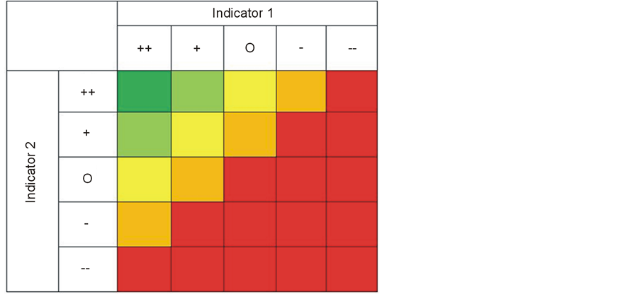
Figure 1. Schematic example of a matrix.
The area-wide collation of the indicators is carried out using a grid. The grid size can be adapted to the conditions of the sample area. In order to achieve a workable and sufficiently detailed recording, an edge length of 50 metres has been chosen. When edge lengths are well above 50 meters, the heterogeneity within the grid can be too large and thus falsify the results. Grid sizes well below 50 meters are recommended only for very small sample areas, as the acquisition effort increases considerably.
For the development of a method, first of all factors relevant for urban climate must be categorised with regards to their detectability. For this purpose, a subdivision is made into “on-site”-mappable, “derivable” and “measurable or determinable” climatic factors. The “local” factors can very easily be recorded by laymen (e.g. degree of soil sealing). The “derivable” factors can be inferred from the “on-site” factors, meaning that no separate reporting is required. The “measurable or determinable” factors, however, cannot be adequately recorded on a site visit. The empirical investigations necessary for an area-wide coverage would lead to extensive additional expenses which would increase the cost of such investigations considerably, as well as making it less workable for laymen. However, should these factors already exist from previous studies or other sources, these may be integrated into the matrices in order to reduce the acquisition effort as well as to improve the quality of the results.
The “on-site”-mappable factors primarily include surface properties (degree of soil sealing, surface colour, surface materials) and city structure (building density, distance between buildings, position of buildings relative to the street). In addition to this, characteristics of the vegetation, such as density and type, can also be recorded on-site. Topographic properties can be recorded on-site as well, however most settlements have digital terrain models available, thus one can forgo an on-site survey in this instance.
The “derived” climate factors fall almost entirely within the hydrological surface properties (runoff regime, infiltration capacity, capillary action, percolation rate and evaporation potential). Only the two factors “height structure of the municipal body” and the “surface roughness” can be allocated to the topic of urban structure.
The “measurable or determinable” factors (traffic, air pollution, energy consumption and behaviour of solar radiation incidence) pose the greatest difficulties in on-site data collection, as these cannot be observed on site without further ado. Although some clues can be detected, such as traces of dirt under the window sills or indicator plants, which indicate high solar radiation, these observations are not sufficiently robust and often not widely available throughout the settlement.
The evaluation of factors relevant to urban climate indicates that not all urban climate phenomena can be covered by this data acquisition method. Particularly the topic of air pollution cannot be comprehensively, but rather only partially, covered. The indicators that are assigned to the areas of overheating, water balance and wind field, however, can either be easily collected on-site or be derived from already acquired factors.
2.2. Data Acquisition
The selection of indicators and matrices used can be adapted to the particular area investigated. The following six matrices can be recommended as a basis for most settlements in Germany:
• Density of soil sealing and density of development• Density of soil sealing and surface colour• Density of soil sealing and surface material• Density of vegetation and topography• Type of vegetation and density of vegetation• Topography and surface roughness.
In addition, matrices have been selected so that individual indicators may be used several times in order to ensure the lowest possible recording effort. The survey can be carried out both analogue as well as application-based with a smartphone or tablet PC.
For an analogue survey, the area investigated is divided into areas comprising of approximately ten grids. For each of these sub-areas, a table is created in which the required indicators can be recorded. An aerial image is used to provide better orientation and ordinance of the particular grid. This aerial image may also be used in order to evaluate areas which cannot be easily accessed. However, in this case it is important to pay attention that the aerial image is up-to-date, as old, out-of-date images may lead to misinterpretations. An overlay between the aerial image and the land register can help to proof the currency of the aerial image.
The smartphone-based survey involves a simple questionnaire. First, the particular grid where the user is located is selected from a survey map. In the next step, the predetermined indicators are queried and then stored in a database. This way the final digitalisation process, which is necessary for the analogue survey, is eliminated. The simple querying of each indicator is particularly well suited for laymen, as they are guided through the acquisition process step-by-step (Figure 2).
After data acquisition has been completed, the data is either digitalised by entering it into a spreadsheet, or uploaded from the mobile database. Thus, the indicators can be allocated to each grid of the different matrices in an automated manner, and may be edited for future processing in a geographic information system (GIS).
3. Urban Ecology Indicators
3.1. Evaluation of Individual Urban Ecology Indicators
The evaluation of the individual elements of the matrix is carried out based on their urban ecological properties, as well as by consulting widely available specialist literature. This results in five different evaluation categories that are established as boundary conditions for the development of positive and negative urban climate phenomena.
Very good urban ecological boundary conditions (++):
The investigated grid shows very good climatic boundary conditions, with regards to the object of investigation, and offers favourable prerequisites for a positive occurrence of the phenomenon.
Good urban ecological boundary conditions (+):
The climatic boundary conditions have an overall positive impact on urban climate. The positive occurrence of this phenomenon is very likely.
Satisfactory urban ecological boundary conditions (~):
The probability of a positive occurrence of a phenomenon is small, but also no negative effects are expected.
Poor urban ecological boundary conditions (−):
The emergence of the phenomenon or the positive occurrence of such can be ruled out. The negative occurrence of the phenomenon is very likely.
Very poor urban ecological conditions (−−):
The investigated grid influences urban climate negatively to a considerable extent. The development of a positive occurrence of the phenomenon can be ruled out.

Figure 2. Data acquisition via smartphone.
3.2. Urban Overheating
Urban overheating is caused by anthropogenic reshaping of the landscape as well as the anthropogenic input of energy. The degree of soil sealing is of particular importance here, as a high degree of soil sealing usually results in other indicators to be very pronounced as well.
3.2.1. Degree of Soil Sealing and Density of Development
In the first matrix (Figure 3), the two elements, degree of soil sealing and density of development, are evaluated. The categorisation is carried out in increments of 25 percentage points at a time. For the degree of soil sealing, four soil sealing categories are created. Within a settlement, the first soil sealing category (0% - 25%) usually includes parks, cemeteries and allotment colonies. In this category, there is only a minor amount of anthropogenic reshaping of landscapes, which means that the urban-ecological properties may be positively rated. Within the second category of soil sealing (26% - 50%), typical structures of development are detached, semi-detached and terraced houses. With an increasing degree of soil sealing, characteristics for the urban ecology in this area deteriorate, as in such areas of more heavily sealed soil the surface runoff increases considerably, and the materials used may heat up significantly [8] . The two top categories of soil sealing are very rarely achieved in small settlements, as these seldom include housing types of dense structures (51% - 75%) or extremely compact core areas as well as industrial estates (76% - 100%).
The density of development is divided into five categories, which are based on the different types of development. The different types of construction are no settlement (0%), clustered development (1% - 25%), semidense development (26% - 50%), dense development (51% - 75%) and very high building density (76% - 100%) [9] .
The defining factor for evaluating the density of development is, in addition to the increased thermal storage capacity due to the building masses, the increase in surface roughness. The increase of the surface roughness hinders the air exchange in these areas, which could lead to the generation of a heat island [10] .
3.2.2. Degree of Soil Sealing and Surface Color
Figure 4 provides information on the thermal behaviour of the area investigated. As a rule of thumb it can be said that lighter areas have a much higher albedo than darker surfaces. Thus, dark surfaces absorb a larger amount of sunlight and therefore warm up more [11] . For this reason, lightly coloured surfaces are given a positive value, while dark areas are given a negative value.
In addition to the surface colour, material also plays an important role with regards to warming. Water surfaces represent an exception here, as they have a low albedo, but all the same warm up very slowly. Furthermore, in this matrix it is just the predominant surface colour which is evaluated, which may lead to a falsification of results at this point. For this reason, the results of this matrix are only an indication, and a more detailed on-site inspection is necessary in order to determine the pollution level.
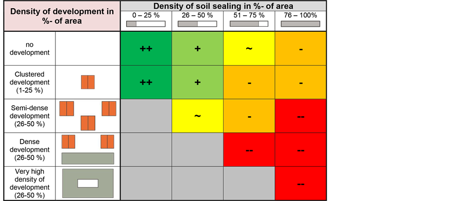
Figure 3. Evaluation of the matrix “density of development/density of soil sealing”.

Figure 4. Evaluation of the matrix “surface colour/density of soil sealing”.
3.2.3. Degree of Soil Sealing and Surface Material
The third matrix is relevant for both urban overheating, as well as for the urban water balance (Figure 5). The materials used in the settlements differ greatly in terms of their thermal conductivity, heat storage capacity and the runoff regime during precipitation [12] .
Due to the large variety of materials used in settlements, detailed data acquisition is not feasible as part of the matrix method. Instead, the materials are divided into five categories, which summarise materials with similar properties. Materials which can percolate into the ground exhibit the best urban-ecological properties, as they usually warm up slowly, have a low runoff coefficient, and make a high rate of percolation and evaporation possible. Areas with crushed stone and gravel have a similar runoff coefficient as materials of the first category, but can warm up more easily when exposed to sunlight, due to their material properties. Water-bound surfaces may differ immensely in terms of their urban-ecological characteristics. Loosely compacted surfaces have a very high proportion of percolation, but with increasing compaction the runoff coefficient increases as well. For this reason, these areas should be subjected to close examination if negative hydrological effects are suspected.
Similar differences in percolation behaviour can occur in the category of pavements and slabs. The fewer the gaps, and the older the pavement or slabs, the worse will be the impact on local climate and water balance. Surfaces of concrete and asphalt exhibit the highest runoff coefficient of the five categories of material, and its mostly grey or black colour additionally leads to unfavourable thermal properties [13] .
For this matrix, the evaluation of the degree of soil sealing is adjusted slightly. Areas with a high degree of soil sealing are no longer automatically rated to be negative. The urban ecological characteristics of the first two surface material categories can still have a positive effect on the urban climate even at a high degree of soil sealing.
3.3. Urban Water Balance
Anthropogenic reshaping of landscapes has a massive effect on the urban water balance. The previous matrices already provide indications of this, as surface materials and the degree of soil sealing have a significant impact on the runoff coefficient.
Density of Vegetation and Topography
The runoff regime of precipitation, and therefore also the urban water balance, are not only influenced by artificial surface materials, but also by vegetation and topography. When comparing areas of identical surface material, the runoff coefficient is significantly higher on a gradient than on flat terrain [14] . For this matrix (Figure 6), the topography is divided into four categories, which range from flat to rough terrain, and from slight to steep gradients.

Figure 5. Evaluation of the matrix “surface material/degree of soil sealing”.
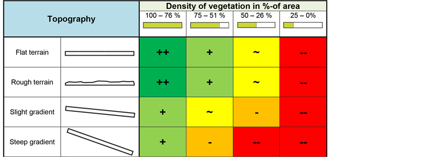
Figure 6. Evaluation of the matrix “surface colour/density of soil sealing”.
During precipitation, vegetation acts as a water barrier which prevents a superficial runoff. Furthermore, plants positively influence the urban climate due to transpiration [15] . The density of vegetation is recorded in the same way as the degree of soil sealing, taking 25 percentage point steps at a time. The reason for this rather rough division is that in practice, considerable discrepancies are possible depending on the time of year and the occurrence of certain plant species.
3.4. Urban Wind Fields
Urban wind fields in settlements present a very complex area. Firstly, differences in local air pressure can lead to small-scale changes in air circulation (surface winds) between the settlement and the surrounding areas, but also within the settlement itself. Secondly, urban development leads to an increase of surface roughness, which results in a reduction of the speed of wind [16] .
3.4.1. Type of Vegetation and Density of Vegetation
Of particular importance to the urban climatic situation of a settlement is the location of cold and clean air forming regions. Using the determined indicators, an extensive investigation into cold air formation cannot be performed, however areas may be derived which carry a high potential of generating cold air. The potential of an area is mainly determined by the thermal properties of the surface material (thermal conductivity and thermal capacity) as well as existing vegetation [17] .
Indicators used in this matrix (Figure 7) are the ones of the density of vegetation as well as the type of vegetation. Type of vegetation is divided into four categories, which are evaluated against their potential for the occurrence of cold air formation. The vegetation type with the highest potential for cold air formation is open spaces with low vegetation (e.g. grass or meadows). Open spaces with groves or shrubs are classed as being slightly inferior in terms of their potential for cold air formation. Woodland areas have a low cold air potential, as the air in the trunk spaces only cools down marginally during the night. Any cold air in forest areas is generated above the canopy. The worst type of vegetation, with regards to the generation of cold air, represents individual plantings such as roadside vegetation [17] .
3.4.2. Topography and Surface Roughness
Cold air formation areas have a positive impact on urban climate. However, its impact on the area is significantly limited if there is no appropriate runoff for the cold air. To ensure that a settlement can benefit from an optimum supply of cold air flows, urban ventilation paths are necessary. Ideal conditions for urban ventilation paths are surfaces that emit very little heat over night, are on a downward gradient towards the settlement and possess a very low surface roughness to insure that the cold air flow is not slowed down or diverted [18] .
In this matrix (Figure 8), the combination of topography and surface roughness is examined in order to identify grids which could act as urban ventilation paths. The surface roughness is divided into three categories (low, medium, high) and is derived from the types of vegetation and density of development. Due to the sensitivity of cold air currents, this analytical method can only provide first indications and could help identify potential areas where further analysis may be worthwhile.

Figure 7. Evaluation of the matrix “type of vegetation/density of vegetation”.
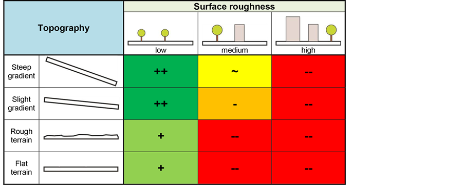
Figure 8. Evaluation of the matrix “topography/surface roughness”.
4. Overall Evaluation of the Urban Ecology
4.1. Urban Ecological Point System
The results of the individual matrices only allow the assessment of an individual object under investigation. An overall urban ecological evaluation of critical areas, or areas with potential, is impossible to be obtained with this approach alone. To achieve such an overall evaluation of the entire investigated area, the results of the matrices can be transferred into a points-based system. The points-based system is based on the five categories of urban-ecological boundary conditions and extends from +2 points (very good ecological boundary conditions) to −2 points (very poor urban ecological boundary conditions). If the six matrices are used, then the maximum and minimum amount of points given for each grid will be +12 and −12 points respectively.
The five evaluation categories are kept the same, in order to ensure consistency in the selection and specification of colours used in the evaluation of the individual matrices and overall evaluation. Thus, for each evaluation category there will be a range of five points.
4.2. Visualisation
The clarity and interpretability of the matrices is significantly improved by the selection and specification of map colours and the reference to the area within the graphic representations. Generally, any method may be used for the representation of the mapping results. The results can be represented using, among others, CAD and graphical software. These programmes are very popular and offer a wide range of visualisation options.
However, the ideal method of choice for visualising the matrix method is represented by geographical information systems, as they offer its users many advantages. In a geographical information system, the automated logical interconnection of the matrices and the individual grids make a quick and simple visualization of the results possible. Other advantages are the ability to link different data sets in order to analyse them, conduct spatial analyses and perform specific queries according to selected combinations of criteria. By using such queries, grids can be very easily and quickly selected which, for example, have a negative rating in both the matrix “vegetation density and topography”, as well as in the matrix “degree of soil sealing and surface material” in order to specifically highlight areas showing critical properties for the urban water balance. If boundary conditions have changed in any way (e.g. new buildings), then these changes can be easily incorporated into the GIS database, resulting in the presentation of results to be automatically updated.
In general, aerial photos should be used as a base map for visualisation, as these make it much easier to connect it to the data collected on-site, as well as making spatial orientation possible. If a local authority is already maintaining a regularly updated GIS-system, then it is possible to replace the base map with other maps (e.g. land development plans) for individual queries, or extend it with additional information.
4.3. Recommendations
After the collection and presentation of urban ecological problem areas has been completed, recommendations may be inferred from these results. Besides highlighting areas displaying very poor urban ecologic conditions, it will also be possible to identify areas with good boundary conditions in almost all local authorities. For this reason, a sub-categorisation into three different zones can be carried out.
Protected zones:
Protected zones are areas which show predominantly good to very good urban ecological boundary conditions and have a positive impact on the local climate. Urban development that can adversely affect these conditions should be avoided in these zones.
Transition zones:
Transition zones neither have a clear negative, nor a strong positive effect on the urban climate. Since this classification is, however, based on the overall evaluation, individual objects of investigation within these zones may still show very strong positive or negative characteristics. A differentiated analysis of the individual objects of investigation must be carried out in these zones in order to identify possible negative influences and take specific measures to improve them.
Redevelopment zones:
The greatest need for action is in the redevelopment zones. These zones show negative characteristics in all three major categories (overheating, water balance and wind field). It can be assumed that these areas have a significant negative effect on the urban climate.
5. Conclusions
The matrix method fulfils the aim of developing a method which allows for urban ecological characteristics within a small settlement to be collected. It is, however, difficult to estimate the exact amount of time and effort saved, compared to complex modelling or empirical data acquisition, as influencing factors are very diverse. These range from the obvious factors such as the size of the settlement, or the amount of matrices, to the base maps available for the acquisition.
The results of the matrix method can be used by communities to identify urban ecological problem areas or areas with positive potential within the settlement. The results of the individual matrices may be used to develop these areas further. The demographic change is a big problem for many small German settlements. The superannuation and the suburbanization cause a high vacancy rate in the settlements. The settlement developer can use the results from the matrix-method to identify areas with a strong urban overheating to suggest controlled demolishing of vacant building to improve the urban climate. Further the results can be used in the planning process of public open spaces. The matrices for the urban overheating and the urban water balance can show which effect a changed degree of soil sealing would have for the urban ecological situation.
Before costly measures are taken, these areas need to be selectively re-examined with regards to the suspected phenomena. The target-oriented application of measurements or modelling is significantly cheaper than a large-scale investigation performed without the matrix method.
It is, however, not possible to infer general recommendations for every settlement from this method, because sensible recommendations should be tailored as closely as possible to the specific target area. Hence, a more detailed on-site investigation is indispensable for this.