Experimental and Numerical Study of Dilute Gas-Solid Flow inside a 90° Horizontal Square Pipe Bend ()
1. Introduction
The research, optimal design and malfunction diagnoses of pneumatic conveying systems require a fundamental understanding and detailed information of both the gas and particle phases. It is common for a conveying mill duct system to incorporate 90˚ bends for changing the direction of the particulate flow within a limited space. Gas-solid flow inside 90˚ bends is complex and chaotic and perhaps for this reason is not completely understood. There are many of documented experimental and numerical studies relating to gas-particle two-phase flows in channels and ducts involving curved 90˚ bends.
Sharma [1] developed a particle tracking direct numerical simulation code to carry out the large-scale turbulent flow and particle transport computations on serial and parallel computers. Fairweather and Yao [2] studied numerically three sizes (1, 50, and 100 µm) of particle dispersion in fully developed turbulent duct flows at three Reynolds numbers up to 250,000. Humphrey et al. [3] reported the first comprehensive air flow velocity measurements using LDA for a square sectioned curved 90˚ elbow bend.
Mekhail et al. [4] conducted CFD simulation of gassolid two-phase flow in a 90˚ bend. predicted the gas velocity vectors. They adopted a computational fluid dynamic code (CFX-TASC flow) for the simulation of the flow field inside the piping and for the simulation of the particle trajectories. They conducted comparison between the results with those presented by Yang and Kuan [5]. Particle trajectories inside 90˚ square bend were predicted using Lagrangian particle tracking model [6]. Also, the effect of presence of solid particles on the velocity field and the erosion pattern using Finnie’s erosion model was studied. Mossad et al. [7] summarized the numerical and experimental investigations of turbulent air flows inside a right-angled sharp 90˚ elbow bend. They compared the CFD predictions of mean velocity profiles of the air flow inside the sharp 90˚ elbow bend against the experimental results obtained using Laser Doppler Anemometry (LDA). Njobuenwu et al. [8] studied turbulent gas-solid flows in square ducts with a 90˚ bend numerically using an Eulerian-Lagrangian approach coupled under the assumption of one-way coupling using a stochastic approach based on a random Fourier series method.
Cheng and Wang [9] developed a model for the impaction efficiency of aerosol particles in 90˚ bends; based on an analytical laminar flow solution and gave the separation efficiency as a function of the Stokes number and curvature ratio. Crane and Evans [10] performed numerical calculations to predict the behavior of aerosol particles in laminar flow in 90˚ bends. Cheng and Wang [11] re-examined the separation of particles in the bends. They concluded that in the laminar flow regime, the particle separation was mainly a function of Stokes number and flow Reynolds number (Re) for curvature ratio between 4 to 20.
A numerical study was done by Keating and Nesic [12] to investigate the erosion-corrosion in a three-dimensional square-sectioned 180˚ U-bend using lagrangian tracking model for simulating the particle motion and three models for predicting the erosion rates, Finnie’s model, Bergevin’s model, and Nesic’s model.
Hence, it is needed to create a whole picture of the dilute phase gas-solid flow behavior and the characteristics in 90˚ duct bend. An understanding of the role of particle properties such as the size, and size distribution or erosion pattern will probably provide the ultimate solution to the problem. However, it is very difficult to quantify the properties such as particle size distribution, particle concentration and so meas urable bulk properties associated with gas-particle interactions.
The present paper documents an experimental and numerical study of dilute-gas solid flow in a horizontal 90˚ bend with a uniform cross-section. Under the assumptions that the solids at dilute concentration have a negligible contribution to gas-phase turbulence, experimental measurements of gas and solids flow properties are performed separately. For the gas-phase, velocities are measured using a three-hole probe. For the dispersedphase, burning sticks of incense are utilized to provide visualization of solids motion and their distribution inside the duct. Numerical simulations are performed for the same flow condition. Validation of the model settings are achieved by repeating a published flow case.
2. Test Rig Facility
Figure 1 shows a schematic diagram of the test rig designed with the objective of handling the research activities of the main transport mode, i.e., dilute phase conveying. It mainly consists of an open supply hopper with slide gate valve, number of conveying pipes with a transparent 90˚ bend that form an open-circuit pneumatic conveying line. In addition, a cyclone separator involved with an air-lock valve is placed after the piping system in order to separate the solids from the flow at the exit of the line. At the end of the conveying line, a high pressure centrifugal fan provides the suitable pressure drop needed for the air flow.
The test setup consists of three square sectioned pipeline ducts of the same cross-section area (0.15 m × 0.15
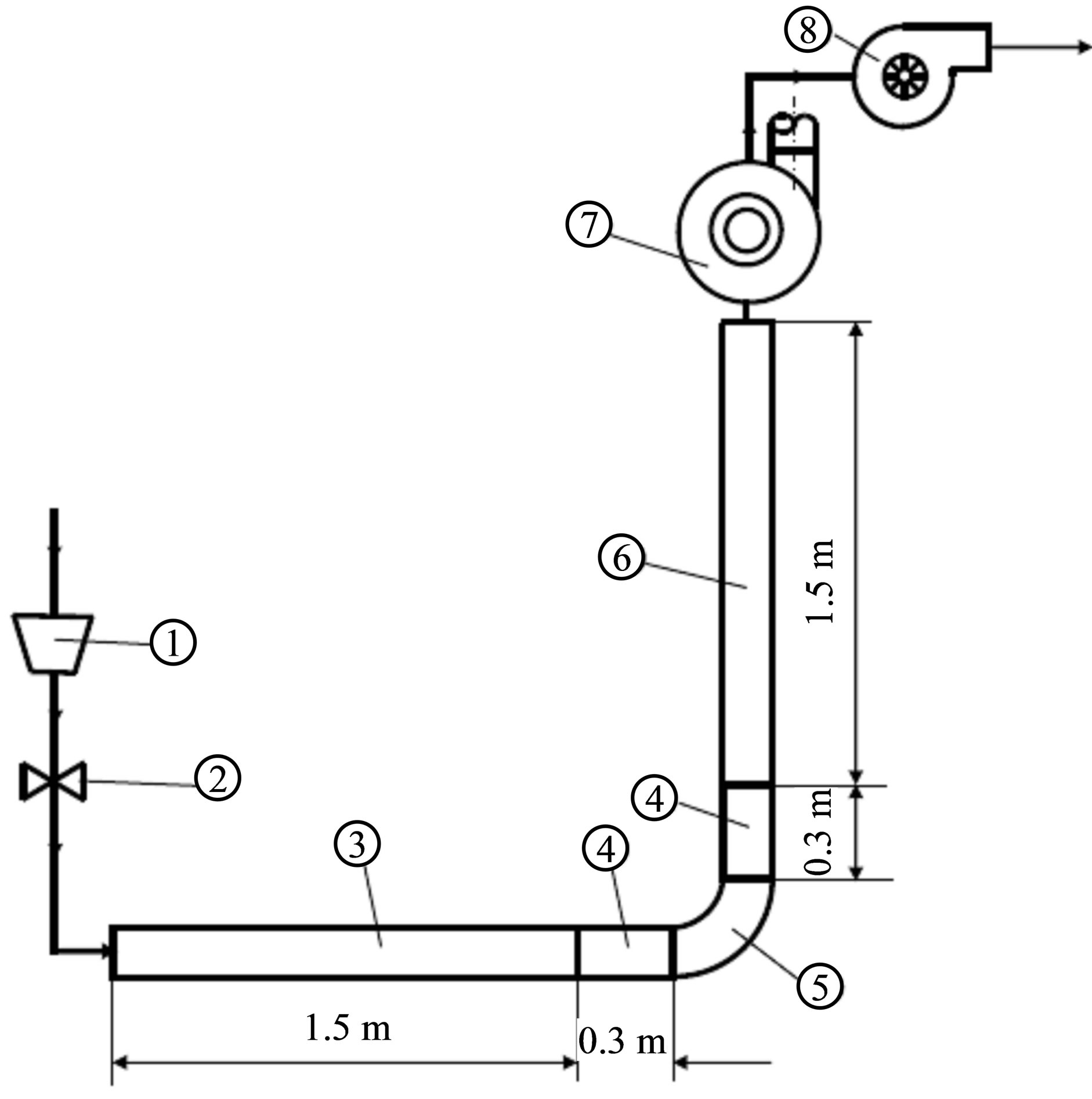
Figure 1. Schematic diagram of the test rig. 1: Supply hopper; 2: Slide gate valve; 3: Upstream duct; 4: Duct joint; 5: 90˚ duct bend; 6: Downstream duct; 7: Cyclone separator; 8: Centrifugal fan.
m) and each has a length of 1.5 m. The pipes are mounted horizontally in 90˚ angle and are connected by a 90˚ bend. The bend is 3 mm in thickness and is made of Perspex. The bend and the two duct joints are perforated, as shown in Figure 2, vertically to the direction of the stream to allow doing the required measurements.
2.1. Gas Phase and Velocity Measurements
The measurement of air velocity as well as static pressure is very important for the present study in order to know the flow pattern, the air velocity distribution at different sections and identify the zones of flow separation; if exits. For measuring purposes; a three-hole probe; Figure 3, is used for velocity measurements of the gas phase only.
Velocity measurements are taken at the vertical plane of the 90˚ duct bend at various locations in the duct’s streamwise direction. At each plane, with the aid of a traversing mechanism, the vertical measurements are taken with an increment of 0.075 m in the upstream and downstream square pipes and of 0.05 m in the 90˚ square bend and the horizontal measurements are taken with an increment of 0.025 m in each pipe. At the bend section, velocity is measured at five locations from 0˚ to 90˚ at 15˚ intervals as shown in Figure 4.
2.2. Solid Phase and Flow Visualization
The knowledge of mean velocity profile of gas flow is required to get an insight of the trajectories of the particles, which represent the solid phase flow within the gas
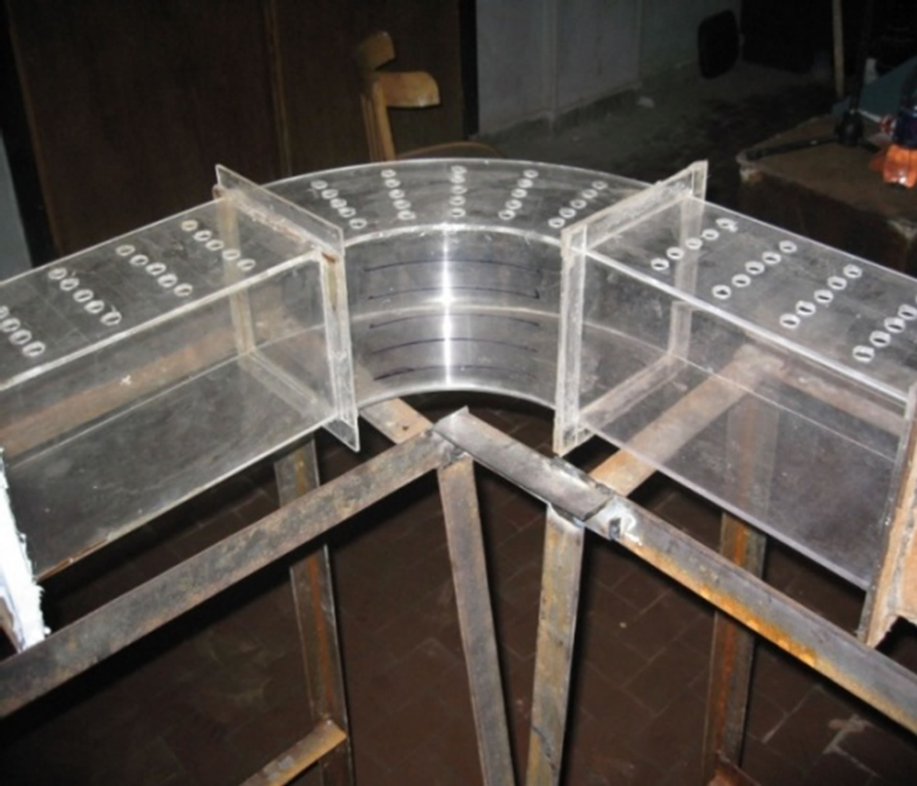
Figure 2. Perforated 90˚ bend and the two duct joints.
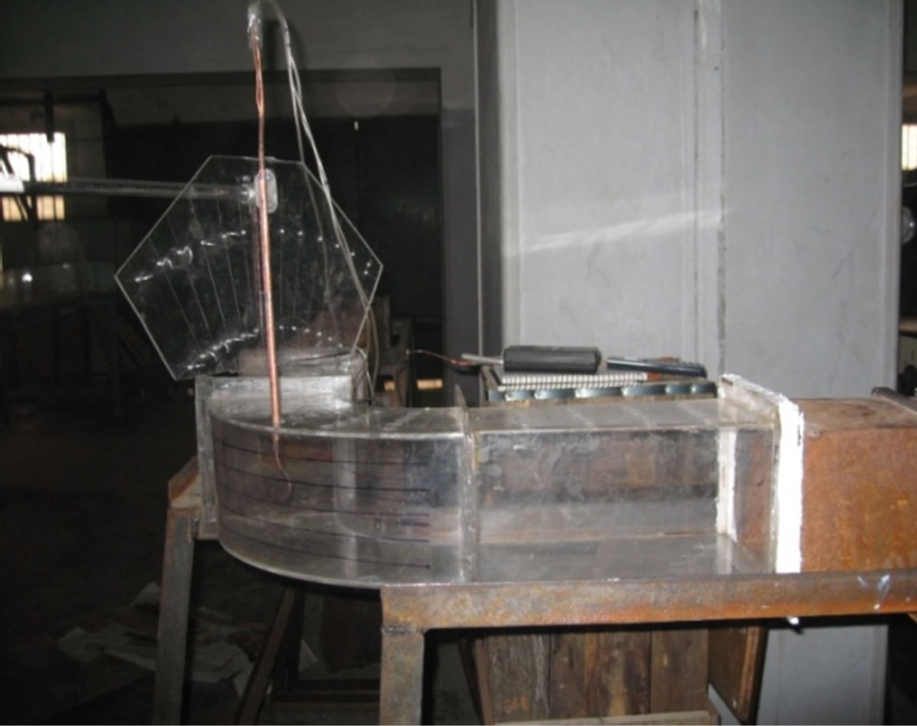
Figure 3. A photograph of the 3-hole probe.
phase. This helps us to obtain an overall picture of the flow particles inside the bend, get a deeper understanding of the flow phenomena and determine the parameters that control and govern particle trajectories and impacts with the bend wall. Hence, the erosion could be analyzed.
As the bend is made of a transparent thermoplastic (Perspex), the flow pattern could be visible by introducing sparks caused by burning sticks of incense within the air flow inside the piping system. A digital camera (Sony DSC-W310 Cyber-shot 12.1 Mega pixels) is fixed in a specific position to take photos of the flow process. Photos of the flow process are taken in a darkened room to make the sparks more visible and detectable. The sparks represent the particles (solid phase) flowing with the gas phase.
3. Numerical Simulation
With the increase of computer power and advancement of commercial modeling software, computational fluid dynamics (CFD) technique is gradually becoming an attractive tool to study turbulent gas-particle flow problems. CFD has the capacity of providing the “microscopic” or “local” information, for instance, the maximum and minimum gas and particle velocity, local particle concentration and individual particle trajectory [13]. Another feature of CFD approach is the graphical presentation of the flow geometry, velocity, pressure, erosion pattern and particle concentration fields.
3.1. Gas Phase
Using a commercial CFD software CFX-2.9.0, the governing equations, Equations (1) and (2), of mass and momentum of the gas phase are numerically solved to get the flow fields and velocity vectors of the gas phase;
 (1)
(1)
 (2)
(2)
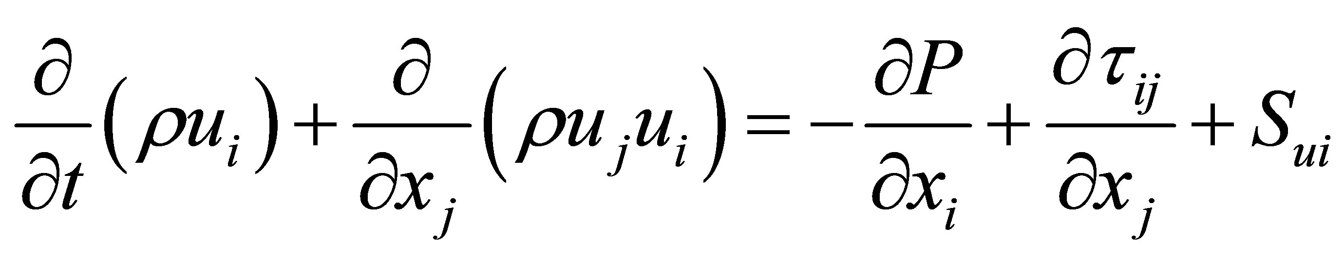
In the above equations, ui represents the velocities in the xi-coordinate directions, p is the static pressure, r is the density, ty is the viscous stress tensor and the S terms are additional source terms. Assumptions made in formulating the tracking model are listed in [14].
The governing equations are discretised using finite volume approach and the grid generator employs a multigrid linear solver to solve the dicretised equations using upwind difference. Recent, comparisons between CFD and the experiments have shown that the standard k - ε model is capable of predicting accurately the important global performance indicators, such as the entrainment and pressure lift ratios, and that the main difference between turbulence models lies in their prediction of local flow structure; Fan et al. [15]. The standard k - ε model is used to predict the turbulence in the straight and bend ducts. The computational domain starts 2D upstream the bend entrance and extends 2D downstream the bend exit. Uniform velocity was imposed at the downstream duct inlet plane of the bend with wall boundary conditions imposed on the top and bottom and also along the sides of the 90˚ square duct. The solution procedure of finite-volume descretization scheme, is solved over one grid system that has a cross-sectional cell density of (ID = 45, JD = 45, KD = 135) or 91125 cells shown in Figure 5.
In the current study, air is used as the carrier fluid and is flowing at a bulk velocity (Vb) of 9.6 m/s, the Reynolds number based on the bulk velocity, hydraulic diameter of the square cross-section and kinematic viscosity of air is (Re = 1.708 × 10⁵) and the pressure at the outlet is 101,325 Pa.
Moreover a grid independent test is carried over using three grid system of (ID = 30, JD = 30, KD = 90) or 81,000 cells and the second one with a a mesh size of (ID = 30, JD = 30, KD = 90) or 273,375 cells and the third one is finer with a mesh size of (ID = 60, JD = 60, KD = 180) or 648,000 cells. The fine and medium cases showed the same results.
3.2. Solid Phase
The most widely applied method available to determine the behavior of the dispersed phase is to track several individual particles through the flow field. Each particle represents a sample of particles that follow an identical path. The behavior of the tracked particles is used to describe the average behavior of the dispersed phase. This
method is called separated flow analysis [16]. The separated flow analysis has been implemented as a Lagrangian tracking model to characterize the flow behavior of a dispersed phase and is optionally available in the CFX-TASCflow software.
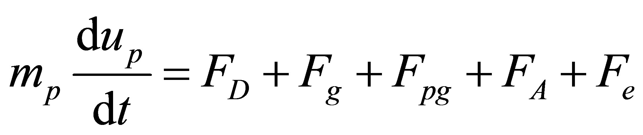
The forces acting on the particle which affect the particle acceleration are due to the difference in velocity between the particle and fluid and due to the displacement of the fluid by the particle. The equation of motion for such a particle can be written as:
 (3)
(3)
where, mp is the particle mass, subscript p represents particle properties and the subscripts D, g, pg, A and e respectively denote the force components arising from drag, gravity, flow pressure gradient, added mass effect and external forces such as electrical field. A detailed description of mathematical models for the force components considered in Equation (3) is available in [16].
Sand particles are used here to represent the solid phase with solids loading ratio of 1.2. To determine the percentage of different sizes contained within the sand, a particle size analysis (sieve analysis) is performed. Particle diameter is analyzed and it is found that there are seven groups of particle diameters, 63 µm, 125 µm, 200 µm, 400 µm, 630 µm, 800 µm and 1250 µm. Figure 6 shows an averaged particle size distribution (by volume) over the sand sample. The particle size distribution versus cumulative volume percentage is also plotted in Figure 7, which indicates that the diameter of sand particles is approximately about 0.2 mm at 10%, and 1.2 mm at 90% of the cumulative mass retained.
4. Results and Discussion
4.1. Gas Phase
The duct has devided into 13 planes as shown in Figure 8. Figures 9(a) & (b) and 10(a) & (b) show experimental
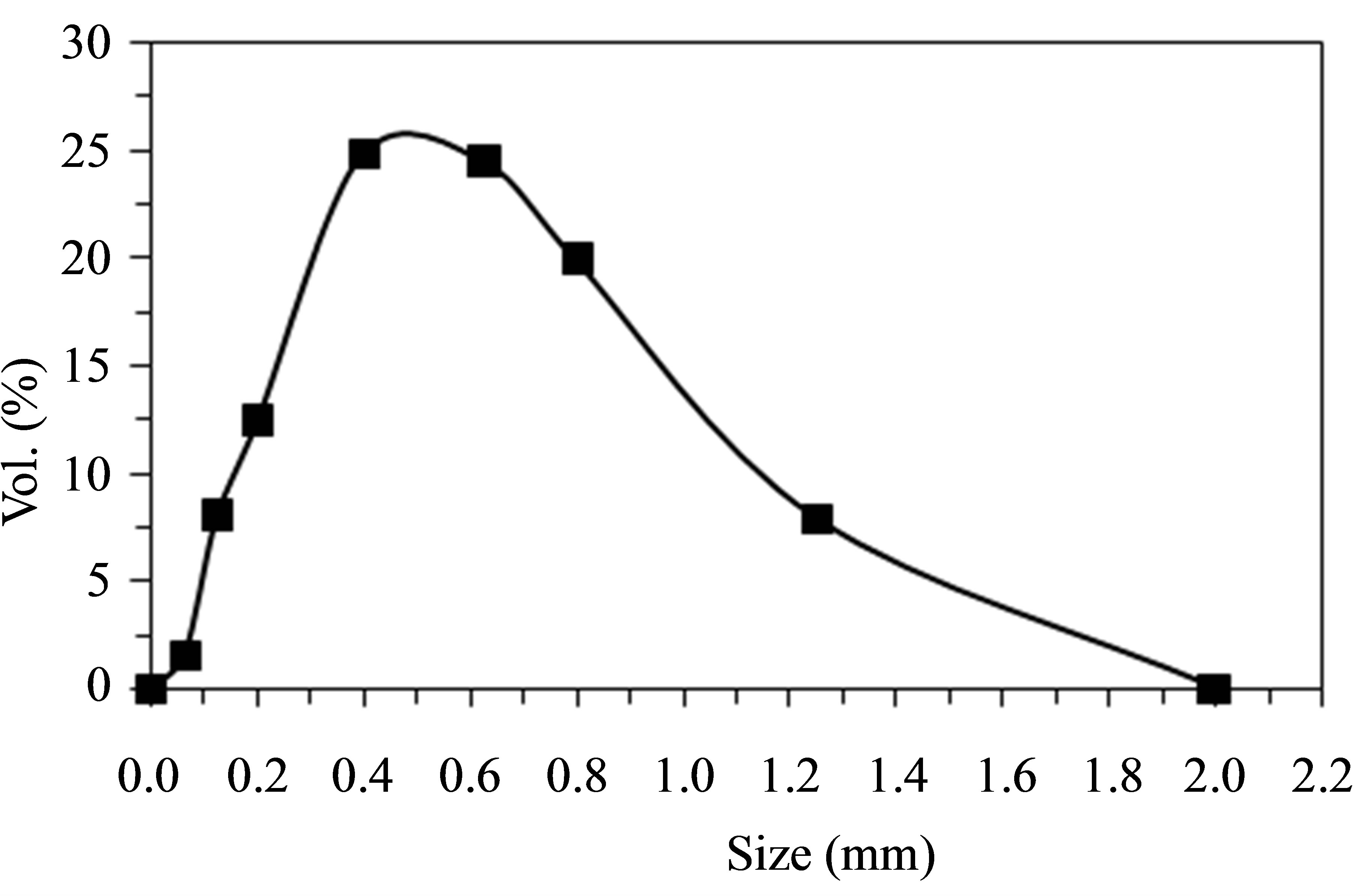
Figure 6. Particle size distribution by volume percentage retained.
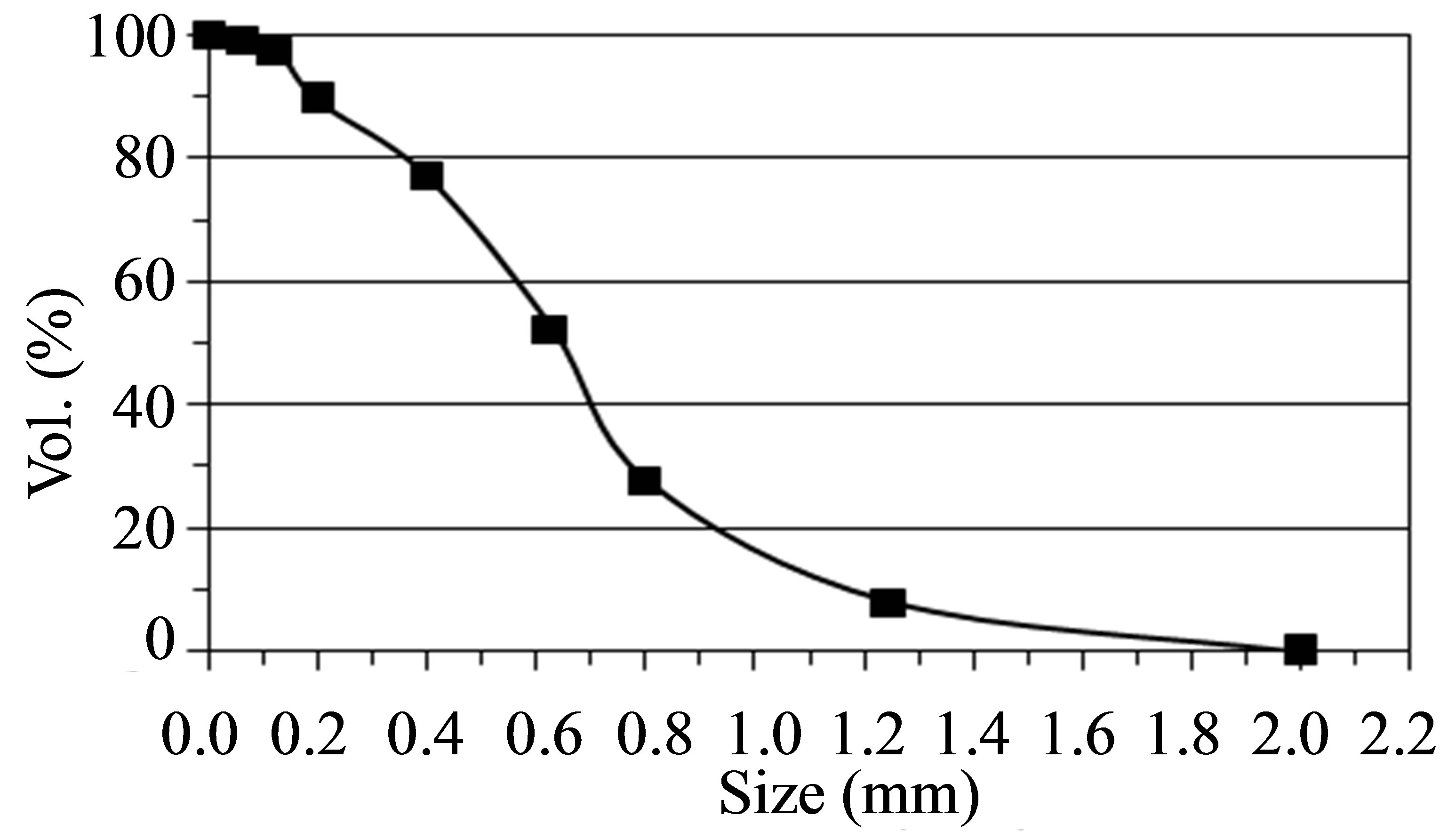
Figure 7. Particle size distribution by cumulative volume percentage retained.
and numerical streamwise velocity profiles of the gas phase at the upstream duct. It may be remarked that the gas is quite evenly distributed which indicates that the flow is symmetric in the straight section and the gas velocity is increased slightly as the gas accelerates from inlet with Vm = 9.6 m/s till nearly 10 m/s at the end of the straight duct. The numerical simulation successfully predicted the acceleration of the gas phase near the inner wall. As the flow advances closer to the bend; Figures 9(c) & (d) and 10(c) & (d), it begins to experience the influence of the bend, which results in the mean velocity profiles becoming slightly skewed, with a small acceleration near the inner wall due to the favorable pressure gradients and a slight deceleration near the outer wall due to the adverse pressure gradients. As seen, the numerical simulation successfully predicted the acceleration of the
gas phase near the inner wall. The presence of the favorable and unfavorable pressure gradients was caused by the balance of centrifugal force and radial pressure gradient in the bend.
The effect of the bend on the flow continues downstream of the bend, Figures 9)e) & (f) and 10)e) & (f), with a reversal of the location of the peak velocity toward the outer wall, leading to a deceleration near the inner wall and an acceleration near the outer wall. This is because of the separation that has occurred in the inner section of the bend due to the adverse pressure gradient.
A comparison between the experimental and numerical results of this study and the results obtained by Yang and Kuan [5] are done. All data are normalized by the bulk air velocity Vb = 9.6 m/s and plotted against a nondimensionalised wall distance;
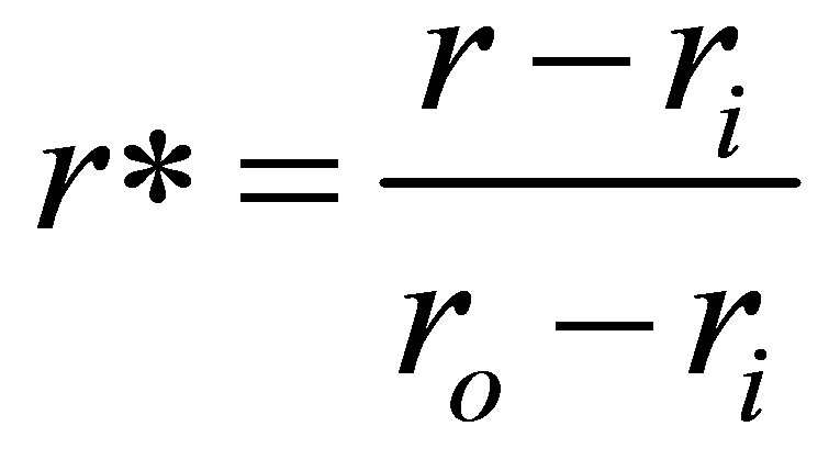 (4)
(4)
such that r* = 0.0 at the inner wall and r* = 1.0 at the outer wall. Figure 11 shows the results at the middle plane section of the 90˚ bend duct (θ = 45˚) and the results show that the behaviour of the present study is in good qualitative agreement with the observation of Yang and Kuan [5].
Figure 11 shows a comparison between the numerical and experimental results in the current investigation and experimental results presented in [5] (Re = 1.708 × 10⁵). It may be remarked that there is a close agreement.
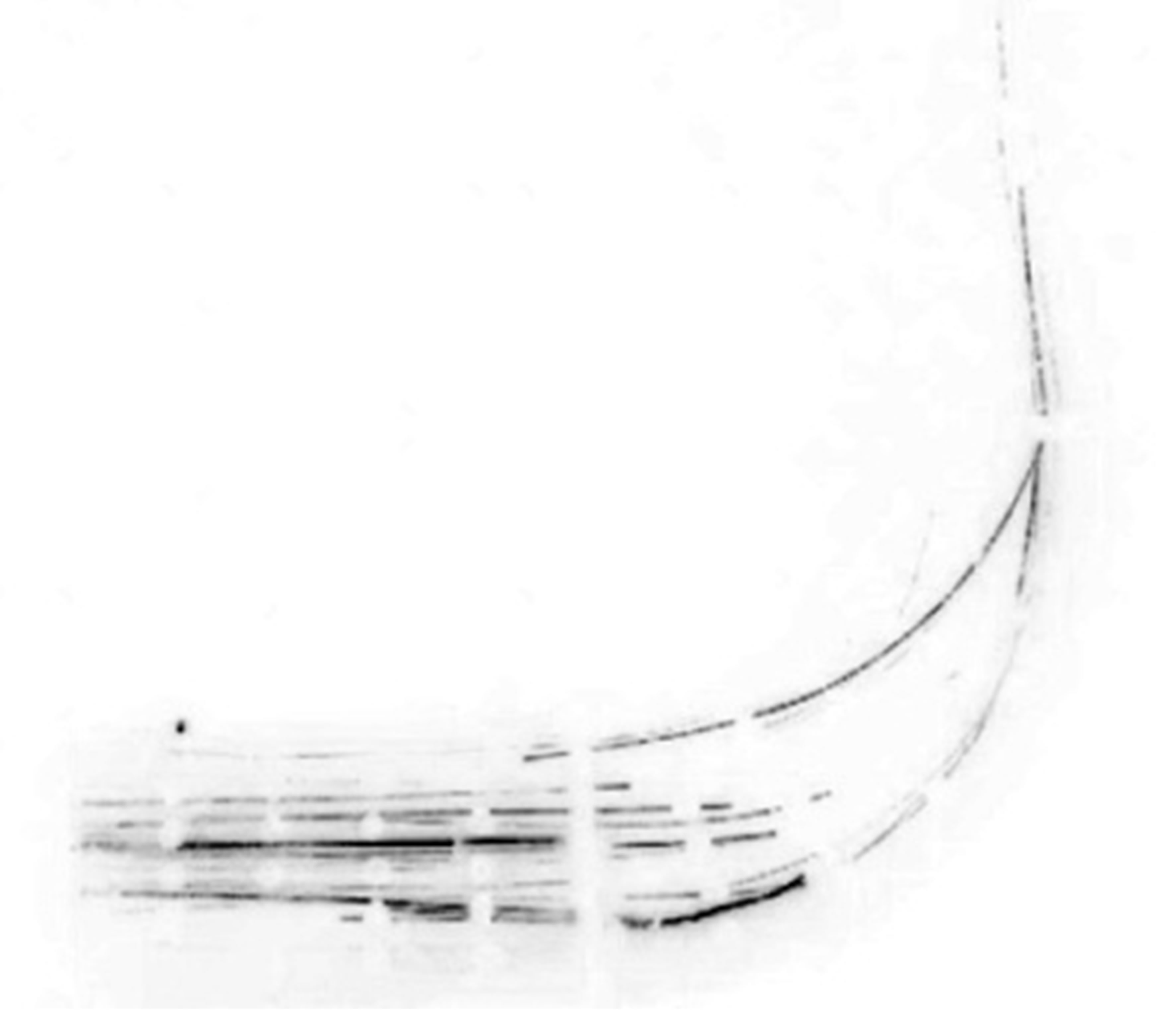
4.2. Flow Visualization
As shown in Figure 12(a), it is obviously seen that the
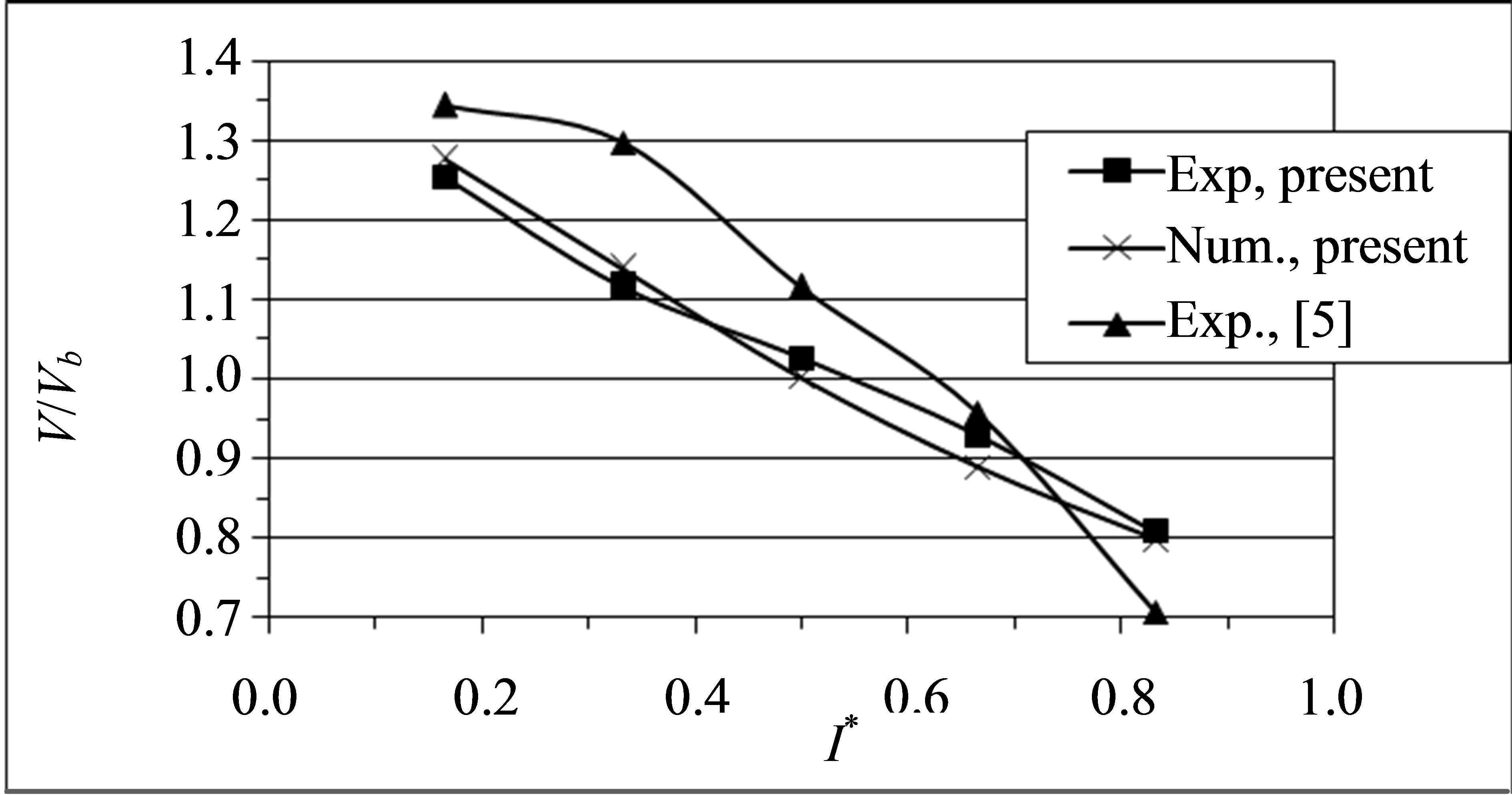
Figure 11. Comparison between experimental, numerical present data and published experimental data of Yang and Kuan [5], θ = 45˚, (Re = 1.708 × 10⁵).
trajectories of sparks in the upstream duct bend are effectively linear. As the sparks are injected with the same initial velocity of the gas, their motion is strongly influenced by that of the gas, with their trajectories similar to those of the gas flow streamlines, which means that the particle streamwise mean velocity profiles are closely similar to the gas streamwise mean velocity profiles and hence the flow is symmetric.
Trajectories of the sparks through the bend section are presented in Figure 12(b). There are two types of trajectories. The first type is where the sparks tend to follow the flow and turning before reaching the outer wall. This type represents the particles with small diameters, since they possessed lower inertia and gained less momentum to overcome the drag of the fluid. The second type is where the sparks don’t follow the flow and hit the outer wall of the bend. This type represents particles with large diameters. This can be explained as the motion of the larger particles is dominated by their inertia and hence they deviate considerably from the gas streamlines within the curved duct.
Figure 12(c) shows the sparks trajectories in the downstream duct bend. Sparks that represent the large particles are subsequently continue to encounter other walls after rebounding from the outer surface of the bend. The high probability of large particles impacting on the walls of the bend is clearly of concern in terms of the wall erosion and pitting effects that occur as a consequence. As the flow travels through the bend it loses its momentum near the inner wall, while gaining momentum near the outer wall.
This behavior is attributed to the flow separation at the inner wall, which arises as a result of the adverse pressure gradient found typically in curved bends. At the exit of the downstream duct bend section, the flow starts to recover from flow separation as the flow starts to re-establish the characteristics of the straight duct flow until it reaches to the fully recovered flow characteristics and is almost assumed to be a fully developed turbulent channel flow.
 (a)
(a)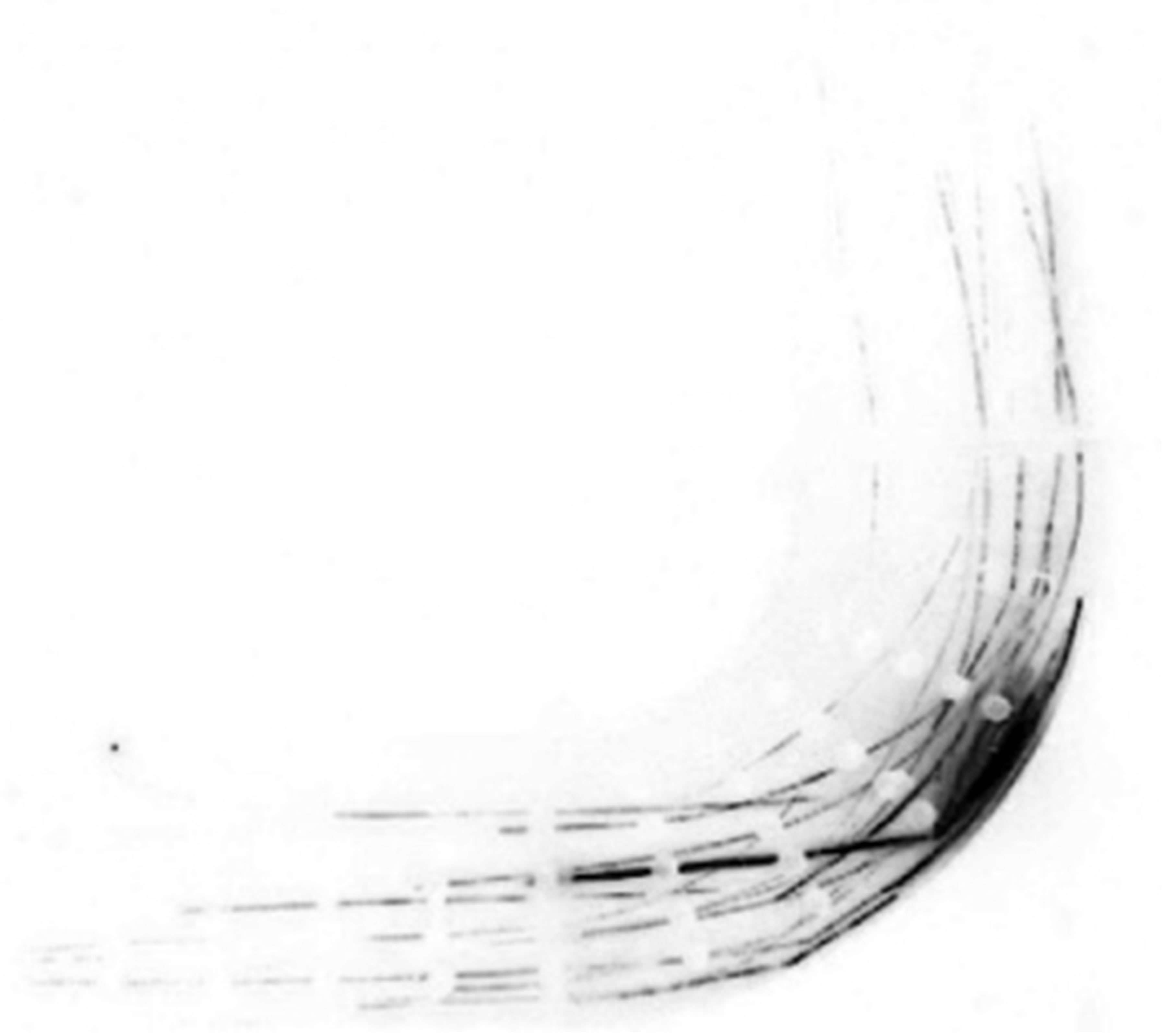 (b)
(b)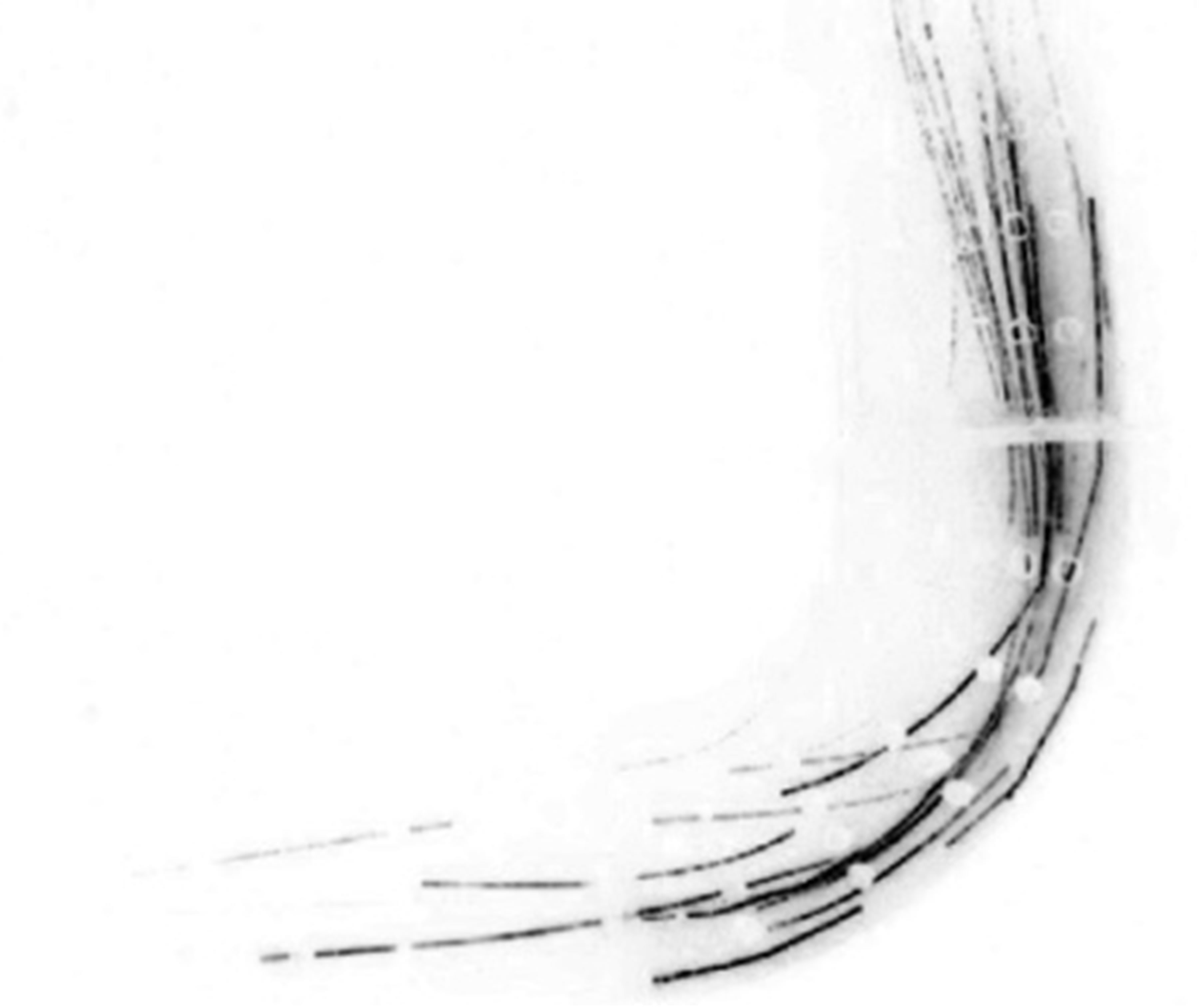 (c)
(c)
Figure 12. Visualization of flow pattern in the 90˚ bend section. (a) Upstream duct; (b) 90˚ Bend section; (c) Downstream duct.
4.3. Solid Phase Simulation
Lagrangian particle tracking with one-way coupling is applied to evaluate particle dynamics within the straight and elbow ducts because solid motion has negligible influence on the carrier fluid flow. Based on the separated flow analysis results, a total of 20,000 particle tracks are calculated for the given particle size distribution and solids loading ratio of 1.2 is used. The total CPU time taken for the solution is (2:40:17) (h:min:sec). The results are presented in Figure 13.
In general, the results obtained numerically using CFX show good qualitative agreement with the visualization figures in Section 4.2. These figures show the trajectories of the particles tracked in a wide range of particle diameters; ranging from 63 mm to 1250 mm, resulting from particle size distribution.
The results show that the particle concentration increases near the outer wall and decreases near the inner wall with the increase of particle diameter; Dp. In an attempt to raise the presence of fine particles in the numerical calculation and hence improve the resolution of the predicted particle tracks in the inner wall region, 100,000 particles have been tracked but this did not result in any noticeable improvement.
5. Conclusion
Measurements are done at different locations using a 3- hole probe to obtain the mean gas flow velocities inside
straight and bend sections. Mean streamwise velocity profiles of gas phase are plotted and they show good agreement with the results published in the literature.
The flow patterns are visualized by introducing sparks caused by burning sticks of incense with the air flow inside the duct system. The results show that particles with small diameters tend to follow the flow due to low inertia and less momentum gained to overcome the drag of the gas, but with the increase in the particles diameter the particles tend to go in straight lines dominated by their inertia. This is a significant parameter that affects the erosion pattern.
Experimental data are used to evaluate CFD simulation results. The mean streamwise gas velocities are predicted and the results are in good qualitative agreement with the experimental data. The particle trajectories are tracked by applying Lagrangian-particle tracking model and the results are in good quantitative agreement with the flow visualization results. It is noted that increasing the number of tracked particles does not result in improvement in the prediction of particle tracks in the inner wall region especially for fine particles.