A Tree Pattern Matching Algorithm for XML Queries with Structural Preferences

Maurice Tchoupé Tchendji¹, Lionel Tadonfouet², Thomas Tébougang Tchendji¹

¹Department of Mathematics and Computer Science, Faculty of Sciences, University of Dschang, Dschang, Cameroon.
²INRIA, Paris, France.

DOI: 10.4236/jcc.2019.71006                

Abstract

In the XML community, exact queries allow users to specify exactly what they want to check and/or retrieve in an XML document. When they are applied to a semi-structured document or to a document with an overly complex model, the lack or the ignorance of the explicit document model (DTD—Document Type Definition, Schema, etc.) increases the risk of obtaining an empty result set when the query is too specific, or, too large result set when it is too vague (e.g. it contains wildcards such as “*”). The reason is that in both cases, users write queries according to the document model they have in mind; this can be very far from the one that can actually be extracted from the document. Opposed to exact queries, preference queries are more flexible and can be relaxed to expand the search space during their evaluations. Indeed, during their evaluation, certain constraints (the preferences they contain) can be relaxed if necessary to avoid precisely empty results; moreover, the returned answers can be filtered to retain only the best ones. This paper presents an algorithm for evaluating such queries inspired by the TreeMatch algorithm proposed by Yao et al. for exact queries. In the proposed algorithm, the best answers are obtained by using an adaptation of the Skyline operator (defined in relational databases) in the context of documents (trees) to incrementally filter into the partial solutions set, those which satisfy the maximum of preferential constraints. The only restriction imposed on documents is No-Self-Containment.

Keywords

Semi-Structured Documents, Preference Queries, Tree Pattern Matching, TreeMatch Algorithm, XML, The Skyline Operator

1. Introduction

Semi-structured documents are increasingly used in the IT community for publishing as well as for exchanging information among applications. Their ever increasing number coupled with the diversity of users and uses encourages the development of ever more efficient techniques for their usage in particular, through dedicated quering languages [2] . Indeed, as for traditional Databases (DB), the need to develop techniques for extracting information from a collection of XML documents (we are talking about XML DB) was very quickly felt, as well to meet the requirements of users/applications needing to explore the web or an XML DB, or for exploiting active documents1 [3] .

Initially, query techniques used in classical DBs had been adapted for use in XML DBs. Unfortunately, this approach is not always appropriate because it only allows to manage the XML subfamily of structured documents2, leaving aside that made up of the large collection of the so-called semi-structured documents. In fact, as opposed to the data manipulated in classical DBs that are structured (we know the schema of the DB), those manipulated in the XML community are generally self-descriptive (semi-structured) i.e., do not have a document model (DTD―Document Type Definition, Schema, etc.). This makes their exploitation and specifically their interrogation through queries very difficult, because of the inexistence or lack of knowledge (by the queries initiator) of their underlying structures: we want to query a document for which we do not know its exact structure (its model). Queries are formulated on the basis of what users believed about the content and/or the structure of the document to be interrogated. Usually, in such situations, in order to maximize chances of obtaining a convincing result, one formulates queries in the most general way to avoid as much as possible having an empty result. In doing so, by the extreme minimization of constraints, one can obtain a very important number of results.

The problems of the absence and/or overabundance of results for a query have also emerged within the community of relational DB (RDB). As a solution, the concept of preference queries was proposed and specific languages have been developed: SQLf [4] , Preference SQL [5] , Preference Queries [6] , etc. This concept has also been adopted within the XML community and languages such as XPref [7] , Preference XPath [8] etc. have been created.

Intuitively, a preference query specifies the user’s desiderata and has two parts: a main condition (similar to a classical query; it is also called exact query or strict query) which aims to select for a RDB a set of n-tuples, or if it is an XML DB, all subtrees of the DB corresponding to the given (tree) pattern, and a preferential part used to specify optional (but preferred) requirements; these requirements can be quantitative or qualitative. Note immediately that an answer to a preference query may not satisfy all or some of the requirements specified in its preferential part, but must necessarily satisfy all those of the main condition.

Initially, the concept of preference queries was motivated among others by the observation that DB users do not generally want to obtain all the answers of a query, but rather, the best or most preferred ones. Subsequently, it was applied in the opposite case (case of an empty answer) to return answers that are “close” to user’s wishes; it’s according to this understanding that they can be qualified as flexible.

Like a RDB, an XML document contains information (data); it also encapsulates a structure that must be taken into account during its querying. In order to transpose the preference concept to XML documents, Sara Cohen et al. in [9] distinguish two types of preferences: those concerning values (the user may prefer results that contain certain values, e.g. low price, best price, etc.) and those related to the document’s structure (the user may prefer results with a certain structure, e.g. existence of a “discount” node or existence in the document’s structure of an arc between “departure” and “arrival” nodes etc.).

The problem addressed in this paper concerns the evaluation of XML preference queries wherein preferences are related only to the document’s structure. Our goal is to propose an algorithm for evaluating such queries by relying on the optimal algorithm proposed by Yao et al. in [10] for the evaluation of exact queries.

The proposed algorithm will use an adaptation of the Skyline operator (defined in RDB [11] ) in the context of XML documents (trees), to incrementally filter the best answers from partial solutions of a query (tree). Finally, it will only return answers that satisfy a maximum of constraints called SkyTrees (see Sec. 3.3): they are the best answers since they are not dominated according to the Skyline operator.

In this paper, 1) we assume as in [10] that the used XML documents are non-recursive3: from this hypothesis, an important property is derived (see Sec. 2.2.1) that allow to considerably accelerate as in [10] , the complexity of the proposed algorithm; 2) to clearly present our approach, we use a sub-language of the query language proposed by Sara et al. [9] ; in fact, we focus only on preferences related to structure called in the following, structural preferences.

Organization of the manuscript: Section 2 presents some concepts related to semi-structured documents as well as the principle of the TreeMatch [10] algorithm. Section 3 is devoted to the presentation of TreeMatchPreference, an extension of TreeMatch to the case of preferences queries. Section 4 presents an experimental study of TreeMatchPreference as well as the prototype built for this purpose. Finally, Section 5 is dedicated to the conclusion.

2. Preliminaries

We present in this section some concepts related to semi-structured documents used in this manuscript. Concepts of exact queries and preference queries are defined more formally. Moreover, the principle of TreeMatch algorithm [10] allowing the evaluation of exact queries is also presented.

2.1. XML Documents, Queries and Evaluations

An XML document is a text file created according to the specifications of the XML standard4. From a purely organizational point of view, it consists of a set of logical structuring units called “elements” or “Tag”; it can be abstractly represented5 by a tree $D=\left(N_d,\mathrm{<mi>\; </mi>}{E}_d\right)$ where N_d is a set of tagged nodes; each node of N_d represents a Tag contained in the document and is tagged by this Tag. E_d is a set of arcs; each arc connects two nodes of N_d according to the existing relationship between tags involved in the (textual) document. For any node x in N_d, function labeld(x) returns its tag. For example, in Figure 1(b) we have a tree representation of an XML document in which a labelled node “a1” represents an occurrence of the “A” tag of the document.

As for XML documents, an exact structural query Q can also be represented by a tree $Q=\left(N_q,E_q\right)$ in which N_q is a set of labelled nodes, E_q a set of arcs each connecting two nodes of N_q; each arc is represented by the pair of nodes it connects. If ar is an arc, function orig(ar) (resp. dest(ar)) returns the source (resp. destination) node of ar. For example, if ar connects n_s and n_d, we write $ar=\left(n_s,n_d\right)$ , and therefore, orig(ar) = n_s and dest(ar) = n_d. There are two types of arcs in E_q: those connecting a parent node to one of his children denoted child (x, y) (or x/y) and those connecting a node to one of his descendants denoted desc (x, y) (or x//y). For any node $x\in N_q$ , function labelq (x) returns its label. Figure 1(a) presents a tree representation of an exact (structural) query containing only parent-child arcs.

Let, $Q=\left(N_q,E_q\right)$ be a query, $D=\left(N_d,E_d\right)$ an XML document, two nodes $n_d\in N_d$ and $n_q\in N_q$ , two arcs $ad\in E_d$ and $aq\in E_q$ :

l We’ll say that, n_d is an occurrence of n_q in D if labeld (n_d) = labelq (n_q). Similarly, we’ll say that ad is an occurrence of aq in D if orig (ad) is an occurrence of orig (aq) and, dest(ad) is an occurrence of dest(aq).

l Let $\psi \mathrm{<mo>\; :\; </mo>}{N}_q\mapsto N_d$ be an application. We’ll say that $\psi \left(N_q\right)$ is a matching of Q in D if the following three conditions are satisfied for all $x\mathrm{,}y\in N_q$ : 1) $x=y\iff \psi \left(x\right)=\psi \left(y\right)$ . 2) $labe{l}_q\left(x\right)=labe{l}_d\left(\psi \left(x\right)\right)$ . 3) if $x\mathrm{<mo>\; /\; </mo>\; <mo>\; /\; </mo>}y\in E_q\Rightarrow \psi \left(x\right)$ is an ancestor of $\psi \left(y\right)$ ; if $x\mathrm{<mo>\; /\; </mo>}y\in E_q\Rightarrow \psi \left(x\right)$ is the parent of $\psi \left(y\right)$ i.e. $\psi \left(x\right)\mathrm{<mo>\; /\; </mo>}\psi \left(y\right)\in E_d$ .

l Q is satisfied in D if there is a match of Q in D. An example of query matching is shown in Figure 1 (blue lines).

As stated earlier, a preference query makes it possible to express requirements some of which are flexible i.e. may not be satisfied when matching. As for exact queries, a preference query can be represented by a tree $\left(N_q\mathrm{,}{E}_q\right)$ in which: 1) The set of nodes N_q is partitioned into two subsets: N_req containing the required or strict nodes―each of them must necessarily have an occurrence in any result of the query―and N_pref containing the preferred nodes i.e. may not have an occurrence in the results. 2) The E_q set of arcs is likewise partitioned into two subsets: E_req containing required arcs and E_pref containing preferential arcs.

A preference query $P=\left(N_{req},N_{pref},E_{req},E_{pref}\right)$ is satisfied on a document D if the exact query $Q_p=\left(N_{req}\mathrm{,}{E}_{req}\right)$ is satisfied on D and elements of N_pref as well as those of E_pref possibly have occurrences in D. Figure 2(a) is an example of a preference query’s tree representation; nodes whose labels contain “?” are preference nodes. The blue lines in Figure 2 show an example of a matching of a preference query on the document of Figure 1(b). Note on this figure that all the required nodes (a, b, c, f) have occurrences; the preference node “d” has some too. On the other hand, the preference node “e” does not have an occurrence in the highlighted solution.

2.2. The TreeMatch Algorithm

Native evaluation approaches of XML queries can be grouped into two classes: class of the one using decomposition-merge-join [12] [13] , and the class of those making a direct evaluation [10] [14] [15] [16] . Among algorithms developed in the second class and handling only non-recursive documents, TreeMatch algorithm developed by Yao et al. [10] has the best time complexity. Generally, in these algorithms, each XML document is manipulated through an index built from an annotation of the latter following the coding (region coding) introduced by Li et al. [17] where each document node is represented by a (start, end, level)

Figure 1. Example of the matching (blue lines) of an exact query (a) on an XML document (b).

Figure 2. Example of matching (blue lines) a preferences query (a) on an XML document (b).

triplet. In the subsequent, we write $Q=\left(N_q,E_q\right)$ the exact XML query to be evaluated on the XML document noted $D=\left(N_d,E_d\right)$ .

2.2.1. Data Structures and Constraints Used in TreeMatch

In TreeMatch, in order to evaluate query Q on document D, a document index based on region coding as indicated above is firstly built. From this index, linked lists T_q, $q\in N_q$ 6 are retrieved: T_q is a linked list of q’s occurrences in D; these occurrences are sorted according to the start component of the triplets annotating the various occurrences of the node q. A stack S_q is associated with each query node q; it will store solutions of the evaluation of the subquery rooted in q.

For each of the T_q lists, a traversing pointer (called TqCurrent) is used to locate at any time the T_q’s element being processed; it initially points on the first T_q’s element. Three primitives are used in TreeMatch: Advance(Tq) which makes TqCurrent point on the next element of Tq, Isleaf(q) which tests if the query node q is a leaf and NumOfChildren(q) which returns the number of children in the query node q: we note $q_i\left(i=0,\cdots ,\left(NumOfChildren\left(q\right)-1\right)\right)$ a q’s child.

An important property of queries handled by TreeMatch―which we also use as a hypothesis―is that of No-Self-Containment i.e. queries nodes’s tags are non-recursive. Indeed, as underlined in [10] , for any query $Q=\left(Nq,Eq\right)$ satisfying this property, for any internal query’s node q, any pair of nodes {x, y} appearing in T_q have no common descendants. As a result, when executing TreeMatch, T_q lists are traversed without going back. Moreover, the matching’s result of subquery rooted on $q\in N_q$ , can be partition into (disjoint) subsets, each containing an occurrence of q. It is this partitioning which allows a compact encoding of the partial solutions (stored in stacks), from which final (global) solution is generated, partition after partition.

2.2.2. Principle

Let $Q=\left(N_q,E_q\right)$ be an exact query, $D=\left(N_d,E_d\right)$ a document. TreeMatch [10] algorithm looks for all matchings of Q in D by recursively calling the find(q) function to determine if the current occurrence of q in Tq (given by pointer TqCurrent) belongs to a partial solution. Where appropriate, the constituents of the said (partial) solution are compactly encoded in stacks associated with nodes of the subquery rooted in q.

Note that, a partial solution is an intermediate result obtained by evaluating a q subquery of Q by matching all the q subquery’s nodes (from the occurrence pointed to by TqCurrent) with nodes in D; it is such that all occurrences of descending nodes of q are descendants of the occurrence of q pointed to by TqCurrent: such D’s node occurrences are said to be covered by the current occurrence of q in T_q7. Partial solutions are likely to be completed further to obtain a complete solutions; if it cannot be done for a given partial solution, it must be properly removed from various stacks. Thus, when ending the query Q processing, the various (partials) solutions are encoded in the different stacks; all that remains is to browse them appropriately in order to synthesize the final solutions and send them back in a more usable form (a tree for instance): GenerateSolution() is the routine that performs this processing in TreeMatch.

3. The TreeMatchPreference Algorithm

TreeMatchPreference is an enriched version of TreeMatch that emphasizes on processing induced by the potential presence of preference nodes in a preference query.

3.1. Principle

Like TreeMatch, TreeMatchPreference is recursive. As input it takes a preference query as well as an index (a set of Tq lists) of the document to be queried. It matches the query with the document (through its index) and returns the best matches, by recursively calling function find (q, TqCurrent, maxPosition)8, to find all possible matches in the subquery rooted in q, from its TqCurrent occurrence. The result obtained on each node is encoded in the stack associated with it.

Function find (q, TqCurrent, maxPosition) is called to determine if the current occurrence TqCurrent of q is a partial solution; its third parameter (maxPosition) makes it possible to ensure that in recursive calls, the only occurrences of descending nodes of q that will be taken into account will be exclusively those whose “end” component of their region encoding is less than maxposition. Indeed, as illustrated in Figure 3 and Figure 4, if we have a query in which qi (child of q) is a preference node, we have to distinguish two situations during the matching: the first one is relative to the case in which several occurrences of qi are covered by the same occurrence of q (see Figure 3), and the second one concern the case in which two consecutive occurrences of qi are covered by two different occurrences of q (see Figure 4). Finally, during the execution of function find (q, TqCurrent, maxPosition), the current occurrence TqCurrent of q is a partial solution if: either q is a leaf, or, each q’s child has a partial solution covered by TqCurrent. Moreover, if q is a preference node, find (q, TqCurrent, maxPosition) must determine whether there are partial solutions that do not include the current occurrence of q: such solutions exist if each of the q’s child has at least a partial solution in the subtrees situated between the current q’s occurrence (TqCurrent) and the one that follows it in T_q. In the following, we qualify such partial solutions as mediocre partial solutions because they do not contain any occurrences of the (preference) query node being processed.

Generally speaking, during the matching process of a query rooted in q, each of its (descending) internal nodes q_i will be process by sequentially applying the same series of operations (grouped in phases, see Figure 5) on each of its occurrences. In particular, we distinguish three phases named phase 1, phase 2 and phase 3; only operations in phase 2 are applied on occurrences of required nodes. In fact, for a preference node q_i, phase 1 (resp. phase 3) look for the existence of mediocre partial solutions not covered by the current occurrence of q_i and belonging to the subtrees preceding it9 (resp. following it); these occurrences must also be covered by the current occurrence TqOc of q (q_i is a q’s child node). In phase 2 however, the processing attempts to find the existence of partial solutions covered by the current occurrence of q_i.

By grouping in phases treatments to be performed to match q_i (a q’s child node), two main cases (see Figure 3 and Figure 4) can be observed: The first case (see Figure 3) concerns the processing of two (many) successive occurrences of q_i (in Tqi) covered by the same occurrence of q: here, the process

Figure 3. Occurrences of q_i covered by the same occurrence of q.

Figure 4. Occurrences of qi covered by different occurrences of q.

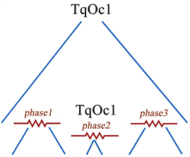
Figure 5. An illustration of the three phases to be observed when processing a query node instance.

performed during the phase 3 processing of the first occurrence coincides with that performed during the phase 1 processing of the second occurrence. In the second case (see Figure 4), two occurrences of q_i are covered by two different occurrences of q: here, we must distinguish the mediocre partial solutions resulting from the processing in phase 3 of the first occurrence of q_i and covered by the first occurrence of q, from the mediocre partial solutions resulting from the processing in phase 1 of the second occurrence of q_i and covered by the second occurrence of q. As mentioned before, it is the maxPosition parameter of function find(), and the fact that lists Tqi are traversed without going back that allows to solve this problem.

3.2. Algorithm

In order to facilitate the management of the mediocre partial solutions resulting from the introduction of preference nodes, update is made to the structures of the tuples inserted in stacks used in [10] .

q being a query node and prefNode(q) (resp. exactNode(q)) designating the set of preferential (resp. required) nodes covered by q, the set of q’s descending nodes is given by: descendingNodes(q) = prefNode(q) È exactNode(q). For instance, for the query sketched in Figure 2(a), we have: prefNode(a) = {d, e} and exactNode(a) = {a, b, c, f }. Let tupq be the encoding of a tuple to be pushed in Sq. tupq consists of five fields and is of the form tupq = (self, parent, exactnode, prefnode, pushCount) in which:

l self contains the occurrence tqcurrent of q.

l parent contains the parent’s occurrence of q in Q; it covers that contained in self.

l exactNode contains sequence $d\mathrm{1,}\cdots \mathrm{,}dk$ of exactNode(q)’s nodes occurrences.

l prefNode contains sequence $dk+\mathrm{1,}\cdots \mathrm{,}dn$ of prefNode(q)’s nodes occurrences.

l Pushcount is a counter incremented when pushing in the stack. This field is used as needed by the cleanStack() function (Algorithm 4) to pop “Pushcount” tuples in the current stack when a partial solution cannot be completed to obtain a complete one.

exactNode and prefNode fields are used exclusively during the generation of the final solution (Algorithm 3).

3.2.1. The TreeMatchPreference Algorithm for Preference Queries

In TreeMatchPreference (Algorithm 1, line 1), TqCurrent initialy point on the first node in Tq1⁰. Then, if q is a preferred node, the phase1 processing is done with the eventual update of the stack associated with q (lines 3-5).

The phase 2 is then triggered with the call of function find(q, TqCurrent, TqCurrent.end) to check if the current q’s occurrence (TqCurrent) can extend some partial solutions to get complete ones. If so, the stack associated with q is updated accordingly (lines 6 - 7). Then, TqCurrent is moved on to the T_q’s next item (line 8) to activate the phase 3 (lines 9 - 15) and the cycle starts again. Algorithm 1 ends with a call to the function in charge of browsing the different stacks to synthesize the final answer (line 16).

Tuples to be pushed in stacks have the form where, “tqcurrent” is the value to be assigned to the self field: this value is either the q’s current occurrence, or a symbolic value denoted Φ if q is a preference node; in this case, one must be either in the phase 1 or else in the phase 3 of the treatment. parent_ is the value to be assigned to the tuple’s parent field: this value is the value of the parent node’s occurrence of q covering tqcurrent, or is equal to the symbolic value “root” if this parent must be located beyond the root (Algorithm 1, lines 5 and 12).

3.2.2. The Find Algorithm for Preference Queries

The new version of the find() function that handles preferences takes three input parameters: find(q, TqCurrent, maxPosition) (Algorithm 2); the first parameter q is the current node of the query being evaluated, the second parameter TqCurrent is either a q’s occurrence, or (in the case where we are in phase 1) the occurrence of his closest ancestor. The third parameter maxPosition is an integer used to set an upper limit on the positions of the nodes that can be processed during the call11.

The different processing phases of q’s occurrences are highlighted in Algorithm 2 via comments. Treatments related to phase 1 are encoded in lines 7 - 10, while those relating to phase 2 are in lines 25 - 27; finally, in lines 29 - 34 we have those relating to phase 3. When partial solutions encoded in stacks cannot be extended to obtain a complete solution, they are popped (Algorithm 2, lines 13 - 15) by using function cleanStack() (Algorithm 4).

Algorithm 1: The TreeMatchPreference algorithm for preference queries.

3.3. The Result Generation Process

Function GenerateSolution() (Algorithm 3) is called to produce an explicit (tree) representation of the final result―consisting of the best answers to the query―from the information encoded in the tuples stored in the stacks.

As mentioned in the introduction, intuitively, a match (a tree) will be more preferred if it contains the largest number of preference nodes’s occurrences. However, note immediately that two matchings (let’s call them r1 and r2) can be incomparable; this is the case if there are at least two query nodes, X and Y, such that exactly one of the two matches, r1 or r2, contains an X’s occurrence and in this case, only the other contains a Y’s occurrence. It is from this observation that we had the inspiration to use an instrumented version of the Skyline operator [11] for the selection of the best answers. In fact, by using this operator, we can define a partial order on the answers so that the best answers are the maximum elements for that order.

Recall that, as defined in RDB, Skyline operator [11] allows to select the best n-tuples of a relational table; it can be briefly, presented as follows: let’s consider a relational table R with schema $R\left(P_1\mathrm{,}\cdots ,P_K\mathrm{,}{P}_{K+1}\mathrm{,}\cdots ,P_n\right)$ and two tuples $p=\left(p_1\mathrm{,}\cdots \mathrm{,}{p}_k\mathrm{,}{p}_{k+1}\mathrm{,}\cdots \mathrm{,}{p}_n\right)$ and $q=\left(q_1\mathrm{,}\cdots \mathrm{,}{q}_k\mathrm{,}{q}_{k+1}\mathrm{,}\cdots \mathrm{,}{q}_n\right)$ in R. For queries in which preferences relate to fields $P_{k+1}\mathrm{,}\cdots \mathrm{,}{P}_n$ , we’ll say that p dominates q and we write $p>q$ , if the following conditions are met:

1) $p_i=q_i$ , for all $i=1,2,\cdots ,k$ ./* required node occurrences coincide */.

2) $p_i\ge q_i$ for all $i=\left(k+1\right),\cdots ,n$ .

3) there are $i\mathrm{,\; <mi>\; </mi>}\left(k+1\right)\le i\le n$ , and $p_i>q_i$ .

By considering the so far manipulated data structures, (see Sec. 3.2), we propose a new definition of the notion of dominance that is more suitable for comparing partial solutions produced during the matching; this notion will allow us to easily synthesize the best answers: they are those which are not dominated.

Definition 1. The dimension of a tuple―Let $tu{p}_q=\left(parent\mathrm{,}self\mathrm{,}{d}_1\mathrm{,}\cdots \mathrm{,}{d}_k\mathrm{,}{d}_{k+1}\mathrm{,}\cdots \mathrm{,}{d}_n\right)$ be a tuple encoded in a stack. The dimension of $tu{p}_q$ noted $dim\left(tu{p}_q\right)$ , is the set of query nodes $q_{d_{k+1}}\mathrm{,}\cdots \mathrm{,}{q}_{d_n}$ for which $d_{k+1}\mathrm{,}\cdots \mathrm{,}{d}_n$ are occurrences: $dim\left(tu{p}_q\right)\subseteq prefNode\left(q\right)$ .

Definition 2. Non dominated Tuple―Let $tu{p}_q=\left(parent\mathrm{,}self\mathrm{,}{d}_1\mathrm{,}\cdots \mathrm{,}{d}_k\mathrm{,}{d}_{k+1}\mathrm{,}\cdots \mathrm{,}{d}_n\right)$ and $tu{p^{\prime }}_q=\left(paren{t}^{\prime }\mathrm{,}sel{f}^{\prime }\mathrm{,}{d^{\prime }}_1\mathrm{,}\cdots \mathrm{,}{d^{\prime }}_k\mathrm{,}{d^{\prime }}_{k+1}\mathrm{,}\cdots \mathrm{,}{d^{\prime }}_m\right)$ be two tuples belonging to the same stack. We say that $tu{p}_q$ dominates $tu{p^{\prime }}_q$ and we write $tu{p}_q>tu{p^{\prime }}_q$ , if $tu{p^{\prime }}_q$ ’s dimension is included (strictly) in $tu{p}_q$ ’s dimension: $\left(\left(tu{p}_q>tu{p^{\prime }}_q\right)\iff \left(dim\left(tu{p^{\prime }}_q\right)\subset dim\left(tu{p}_q\right)\right)\right)$ .

Function GenerateSolution() (Algorithm 3) is similar to its counterpart with the same name in [10] . However, it differs from the latter in that it performs special processing on preference nodes in order to take into account the possible absence of occurrences of such nodes in encoded answers store in stacks. Indeed, among answers stored in stacks associated to preference nodes, only the best (qualitative preference) should be retained. The Skyline operator provided with

Algorithm 2: The find algorithm for preference queries.

the dominance relation defined above makes it possible to make this selection: an answer (a tuple) is retained only if it is not dominated by any other. Function filterSkylineSolution() called in Algorithm 3 is used to incrementally make this selection.

More precisely, function GenerateSolution() (Algorithm 3) performs a preorder traversal of different stacks associated with nodes of the query tree. At each node, it realizes the equijoin of the associated stack and those of her children and stores the non dominated tuples in the same stack (overwrite). Finally, query’s answer is synthesized from the leaves of the query tree and is stored in the stack associated with the root node of the query tree.

Algorithm 3: The GenerateSolution algorithm for preference queries.

3.4. Illustration

This subsection is devoted to a completely illustrated presentation (from the data initialization to the generation of the final solution) of the matching of a preference query (see Figure 6) on an XML data source (see Figure 7). An index T (the Tq lists, Figure 8) is build from the XML data source, and the evaluation function TreeMatchPreference (a, T) is called to match the query with the data source. Notice that, parameter “a” used in the call is the root node of the query (see Figure 6).

TreeMatchPreference starts by examining whether the first occurrence “a1” of “a” in T_a is a solution to the query rooted in “a”. More precisely, the goal is to determine (see Figure 9) if “a1” is the root of a subtree consisting of well-structured occurrences of b, c, f and possibly d and e? If so, the tuple < a1, root, 1> must be pushed in S_a (the stack associated with the query node a).

Algorithm 4: The cleanStack algorithm.Algorithm 5: The joinAndFilter algorithm.

Figure 6. A tree representation of a preference query used to query the data source of Figure 7.

Figure 7. Region coding labelling of the nodes of an update of Figure 1(b).

Figure 8. T_q obtained from the data source of Figure 7.

Figure 9. Evaluation of the query node a.

Knowing that node “a” has a son (node “b”) and that TreeMatchPreference make a call to the recursive function (find()) when matching, the previous question is renewed on the current occurrence “b1” of “b” to examine if “b1” is a partial solution1²? This question is equivalent to this one: “should we push tuple < b1, a1> in S_b?”. Like before, due to the function find() recursion, the question “should we push tuple < c1, b1> in S_c?” is examined (see Figure 9) and the answer is “Yes” since, c is a leaf node and c1 is covered by b1; tuple < c1, b1> is then pushed in S_c (see Figure 10(a)).

After tuple < c1, b1>’s stacking, T_c’s traversing pointer is moved to the next occurrence of c; “c2” then becomes the new current occurrence of “c”. Since c2 is not covered by “b1”, evaluation continues on “d” (the second son of “b”); the current occurrence of “d” in T_d is “d1”. Since d is a preference node, TreeMatchPreference examine if tuple <Φ, b1> can be pushed in S_d? This corresponds to the execution of the so-called phase 1 (Algorithm 2, line 8). As above, the recursion of find() and the fact that e is a preferential node must lead to another test: “should we push tuple <Φ, b1> in S_e?” (see Figure 10(b)). Note that in the tuple <Φ, b1>, the attribute parent is set to b1 (and self = Φ); this reflects the fact that the parent of e does not have any occurrences in the partial solution under construction13.

The test “push <Φ, b1> in S_e?” is positive since e is a leaf (Algorithm 2, line 1); <Φ, b1, 1> tuple is then stacked (see Figure 11(a)) and the T_e’s traversing pointer is moved to “e2”. Since “e2” is not covered by “d1”, the processing continues with the evaluation of f (the next child of “d”), f1 being its current occurrence. The test “push < f1, b1> in S_f?” is performed with a negative answer since f1 is not covered by b1: can’t be pushed in S _f (see Figure 11(a)). The negative answer to the test “push < f1, b1> in S _f?” imposes the deletion (by using function cleanStack) of one tuple (pushCount = 1) in S _e which is “linked” to “b1” in S _d (see Figure 11(b)).

After going through all the lists T_q ( $q\in \left\{a\mathrm{,}b\mathrm{,}c\mathrm{,}d\mathrm{,}e\mathrm{,}f\right\}$ ), TreeMatchPreference will have stored in each stack (see Figure 12) a compact encoding of all solutions (tuples) of the query.

Function generateSolution() is then called to produce the non dominated tuples. To do this, it merges and cleans the contents of stacks by performing at each node the equijoin of the stack associated with it and that of its children; only non dominated tuples are retained. Function joinAndFilter() (Algorithm 5) is used for this purpose.

Figure 13 shows the executing result of function generateSolution() when it is run over the stacks sketched in Figure 12. generateSolution() being recursive and performing a pre-order traversal of the query tree, it is invoked by providing it with the root node of the query. The first merge is made between the S_b and S_c stacks to provide the new S_b stack (dotted in Figure 13). The second merge is made between the S_e and S_d stacks to obtain the stack sketched in Figure 14(a). Note that each tuple of this stack is followed by a pair of binaries (x,y) in which, x (resp. y) allows us to know if the tuple contains (“1”) or not (“0”) an occurrence of a preference node e (resp. d). For instance, for a stack entry containing (1, 1)>, the pair (x, y) is equal to (1, 1); this means that tuple < d4, b3, e4> contain an e’s occurrence (e4 for this case) and a d’s occurrence (d4 for this case). On the other hand, <Φ, b3, e3> (1, 0) indicates the presence (x = “1”) of an occurrence of e (e3 in this case) and no occurrence (y = “0”) of d. A tuple that does not have any occurrences of the preference nodes will have this pair equal to (0, 0).

After merging S_d and S_e, the filter function is applied to the result to remove duplicate tuples as well as to extract those that are not dominated. Figure 14(b) shows the resulting stack; it gives an illustration (on the portion noted [4] ) of the extraction of the not dominated tuple < d4, b3, e4> among tuples { , }. The stack of the Figure 14(b) is finally the one associated with node “d”; it is subsequently merged with S _f. Proceeding as for S _e, we have the new stack S _df (see Figure 15(a)), and finally that of S _af (see Figure 16(b)) which contains only not dominated tuples: these are the best answers sought.

4. Implementation and Experimental Study of TreeMatchPreference

In the previous section, we described TreeMatchPreference together with functions on which it relies upon when evaluating a query. In order to facilitate its

Figure 10. Pushing in S _c (a) and Evaluation of the preference query node d (b).

Figure 11. Pushing <Φ, b1> in S_e and negative answer for test of pushing ( in S _f) (a) and pop of <Φ, b1> from S _e (b).

Figure 12. Stacks storing the encoding of all matches of the query of Figure 6 with the data source of Figure 7.

Figure 13. Merging S_d and S_e followed by S_d’s filtering.

Figure 14. Merging S_d and S_e followed by filtering.

Figure 15. Merging S_b and S_c followed by filtering.

Figure 16. Merging S_df and S_b (a), merging S_bf and S_a (b) followed by filtering.

experimentation with well-known and recommended XML DBs for testing XML query evaluation algorithms, we have developed a platform for the expression and execution of preference queries; it allows us to select an XML data source, define or select an existing query, apply a query to a data source, and then view the best answers resulting from the match. Finally, this platform allowed us to easily experiment with the proposed algorithm by using it for the evaluation of many preference queries on various XML data sources. A summary of the work done for this purpose is presented in the following two subsections.

4.1. XML Databases and Sample Queries

l SigmodRecord.xml contains an index set of SIGMOD registry items (http://www.dia.uniroma3.it/Araneus/Sigmod). The following queries have been applied to this file:

1) “SigmodRecord[/issue[/volume?/15?]/articles/article/authors/author/Sophie Cluet]’’: search all articles of author “Sophie Cluet” belonging to the fifteenth volume’s publication; the fact of belonging to the fifteenth volume of publications is preferential.

2) “/authors[/author/Sergey Brin]/author/Rajeev Meitwani?”: search all articles written by authors “Sergey Brin” and “Rajeev Meitwani”. In the best case, the returned results will have these two authors and in the worst case, only those of “Sergey Brin” will be returned, because “Rajeev Meitwani” is preferential.

l part.xml contains information about products of the Transaction Processing Performance Council (TPC-http://www.tpc.org/tpch/). The following queries have been applied to this file:

1) “table[/T[/INT/P_BRAND/Brand#13?]/P_CONTAINER/SM_CASE]”: this query looks for products from the “SM_CASE” container with a preference over those belonging to the “Brand#13” brand.

2) “table[/T[/P_TYPE/LARGE?][/P_SIZE/10]/P_CONTAINER/MED_BOX?]”: this query searches for size 10 products in any container with a preference for those from the “MED_BOX” container.

l The last experiment file mydata.xml is not part of a repository. It was created by following the XML document fragment of Figure 7 and two queries (“a[/b[/c]/d?[/e?]/f]’’ and “a[/b[/c]/d?[/e]/f]’’) were executed on it.

4.2. An Overview of the Tool Developed for Executing Preference Queries

The main window of the developed prototype is divided into four panels (see Figure 17):

l The upper left panel is used to select the data source to query.

l The lower left panel is used to select an existing query or to edit a new one.

l The top right panel is used to display the best answers.

l The lower right panel displays the tree structure of a selected answer in the upper right panel.

For instance, to query mydata.xml data source, click on the “select file” button (see Figure 17) to select the file to query. Once the file is selected, it is parsed and an index based on region coding is generated. Then, a corresponding tree representation is displayed in the dedicated panel, followed by loading existing queries (related to the selected file) into a drop-down menu (from the same panel). Since these loaded queries are editable, it is possible for a user to completely (re)formulate a new one.

Figure 17. The GUI of the tool developed for experimenting the evaluation of preference queries.

Figure 18. A screenshot sketching the matching process.

When selecting an element (a query) in this drop-down menu, its tree representation is drawn just below. Right next to the drop-down menu, the “Process” button is used to launch the document querying process. Best matches found are displayed on the top left panel (see Figure 18) and the selection of one of them causes the display on the down left panel of its tree representation (see Figure 18).

5. Conclusions

This article focused on importing the concept of preference queries into the XML community. For this purpose, we have proposed TreeMatchPreference which is an algorithm (inspired by TreeMatch [10] ), to evaluate preference queries on an XML data source. The query language used is a subset of that proposed by Cohen and Shiloach [9] in which we have retained only structural preferences.

Inspired by Skyline techniques used in RBD for evaluating preference queries [18] [19] , we proposed a so-called SkyTrees. SkyTrees is the set of best (non-dominated) answers obtained when using TreeMatchPreference to match a preference query on an XML data source.

A short-term work will consist of the full analytical study of the proposed algorithm and its extension to the processing of value-based preference queries.

We also plan to explore a presentation of the proposed algorithms following a grammatical approach inspired by that adopted by Bouchou et al. [20] for XML integrity constraint validation: the expected gain is the fluidity of the presentation (algorithm design would be more modular) and the reduction of the query’s tree traversing time.

Acknowledgements

Authors warmly thank Beatrice Bouchou for suggesting the theme discussed in this paper.

NOTES

*This paper is the extended version of the one titled Evaluation des requêtes avec préférences structurelles sur les documents XML [1] presented at CARI’14.

¹An active document is a document with dynamic parts (nodes) encapsulating queries on other documents. Their dynamic parts (nodes) are supplemented by necessity―at the moment of its use―by executing queries that they encapsulate.

²An XML document is said to be structured if it is valid with respect to a given document model; for example, a DTD, Schema, etc.

³In such documents, no element (Tag) is in the list of its descendants.

⁴http://www.w3.org/XML/

⁵In an abstract document, one can ignore texts and attributes nodes: these are not relevant for the purely structural treatments which interests us in this paper.

⁶In order to simplify the presentation, as long as there is no ambiguity, in the rest of this paper, we will not make any difference between a node and its label.

⁷In general, when a node n belongs to a subtree rooted in r, we say that r covers n; in this case, considering the li’s coding, we have: r.start < n.start < r.end.

⁸From the function find()’s type, we can already note that it differs from the one used in TreeMatch.

⁹As we will see in function find() (Algorithm 2), it is the third parameter (maxPosition) of find() that will discriminate. Indeed, nodes involved in this phase are those whose end components of their region encoding are less than maxPosition.

¹⁰In function find(), we use the routines pHead(Tq) that return the reference of the first element of Tq and dropHead(Tq) which removes the first element of Tq and return the residual list.

¹¹For example, with the call find(q, TqCurrent, 20), only nodes with a value less than 20 in the “start” component of their region encoding will be considered.

¹²Remember that a b_i occurrence of b is a partial solution if and only if there exists an occurrence of each of its sons (here c and d) which are sons of b_i and which are themselves partial solutions.

¹³We are evaluating a mediocre partial solution (see Sec. 3.1) which does not include a d occurrence. We will then examine if there exist a solution which does not include neither a d occurrence nor an e occurrence by considering the tuple <Φ, d1> in which Φ materializes the absence of an occurrence of e in the investigated solution. This confirms the fact that find() evaluates a preference node by considering two alternatives: absent or present, respectively corresponding to treatments grouped in phase 1 and phase 2 in Algorithm 2.

Conflicts of Interest

The authors declare no conflicts of interest regarding the publication of this paper.

References

[1]	Tchendji, M.T. and Tadonfouet, L. (2014) Evaluation des requêtes avec préférences structurelles sur les documents XML. In: Sellami, M., Badouel, E. and Lo, M., Eds., Actes du CARI 2014, Saint-Louis, 333-341.
[2]	Cho, S.R. and Balke, W.-T. (2009) Building an Efficient Preference XML Query Processor. Proceedings of the 2009 ACM Symposium on Applied Computing, Honolulu, 8-12 March 2009, 1585-1586.
[3]	Abiteboul, S. (1999) On Views and XML. Proceedings of the 18th ACM Symposium on Principles of Database Systems, Philadelphia, 31 May-3 June 1999, 1-9. https://doi.org/10.1145/303976.303977
[4]	Bosc, P. and Pivert, O. (1995) SQLf: A Relational Database Language for Fuzzy Querying. IEEE Transactions on Fuzzy Systems, 3, 1-17.
[5]	Kiebling, W. (2002) Foundations of Preferences in Database Systems. Proceedings of the 28th International Conference on Very Large Databases (VLDB), Hong Kong 20-23 August 2002, 311-322. https://doi.org/10.1016/B978-155860869-6/50035-4
[6]	Chomicki, J. (2003) Preference Formulas in Relational Queries. ACM Transactions on Database Systems (TODS), 28, 427-466.
[7]	Agrawal, R., Kiernan, J., Srikant, R. and Xu, Y.R. (2003) An XPath-Based Preference Language for P3P. Proceedings of the 12th international conference on World Wide Web, Budapest, 20-24 May 2003, 629-639.
[8]	Kieβling, W., Hafenrichter, B., Fischer, S. and Holland, S. (2001) Preference XPATH: A Query Language for E-Commerce. Proc. 5th Intern. Konferenz für Wirtschaftsinformatik, Augsburg, September 2001, 425-440.
[9]	Cohen, S. and Shiloach, M. (2009) Flexible XML Querying Using Skyline Semantics. Proceedings of the 2009 IEEE International Conference on Data Engineering, Shanghai, 29 March-2 April 2009, 30-37. https://doi.org/10.1109/ICDE.2009.24
[10]	Yao, J.T. and Zhang, M. (2004) A Fast Tree Pattern Matching Algorithm for XML Query. Proceedings of the 2004 IEEE/WIC/ACM International Conference on Web Intelligence, Beijing, 20-24 September 2004, 235-241. https://doi.org/10.1109/WI.2004.10048
[11]	Börzsönyi, S., Kossmann, D. and Stocker, K. (2001) The Skyline Operator. Proceedings of the 17th International Conference on Data Engineering, Hiedelberg, 2-6 April 2001, 421-430.
[12]	Zhang, C., Naughton, J.F., DeWitt, D.J., Luo, Q. and Lohman, G.M. (2001) On Supporting Containment Queries in Relational Database Management Systems. Proceedings of the 2001 ACM SIGMOD International Conference on Management of Data, Santa Barbara, CA, 21-24 May 2001, 425-436. https://doi.org/10.1145/375663.375722
[13]	Al-Khalifa, S., Jagadish, H.V., Koudas, N., Patel, J.M., Srivastava, D. and Wu, Y. (2002) Structural Joins: A Primitive for Efficient xml Query Pattern Matching. Proceedings of the 18th International Conference on Data Engineering, San Jose, 26 February-1 March 2002, 141-152. https://doi.org/10.1109/ICDE.2002.994704
[14]	Lu, J., Chen, T. and Ling, T.W. (2004) Efficient Processing of xml Twig Patterns with Parent Child Edges: A Look-Ahead Approach. Proceedings of the 13th ACM International Conference on Information and Knowledge Management, New York, NY, 8-13 November 2004, 533-542. https://doi.org/10.1145/1031171.1031272
[15]	Chen, S., Li, H.-G., Tatemura, J., Hsiung, W.-P., Agrawal, D. and Candan, K.S. (2006) Twig2stack: Bottom-Up Processing of Generalized-Tree-Pattern Queries over xml Documents. Proceedings of the 32nd International Conference on Very Large Data Bases, Seoul, 12-15 September 2006, 283-294.
[16]	Jiang, Z., Luo, C., Hou, W., Zhu, Q. and Che, D. (2007) Efficient Processing of XML Twig Pattern: A Novel One-Phase Holistic Solution. 18th International Conference Database and Expert Systems Applications, Regensburg, 3-7 September 2007, 87-97. https://doi.org/10.1007/978-3-540-74469-6_10
[17]	Li, Q. and Moon, B. (2001) Indexing and Querying XML Data for Regular Path Expressions. Proceedings of the 27th VLDB Conference, Roma, 11-14 September 2001, 361-370.
[18]	Tan, K.-L., Eng, P.-K. and Ooi, B.C. (2001) Efficient Progressive Skyline Computation. Proceedings of the 27th VLDB Conference, Roma, 11-14 September 2001, 301-310.
[19]	Bouadi, T., Bringay, S., Poncelet, P. and Teisseire, M. (2010) Requêtes skyline avec prise en compte des préférences utilisateurs pour des données volumineuses. Extraction et gestion des connaissances, Hammamet, 26 au 29 janvier 2010, 399-404.
[20]	Béatrice, B., Ferrari Mirian Halfeld Lima Maria Adriana Vidigal (2011) Attribute Grammar for XML Integrity Constraint Validation. Proceedings of the 22nd International Conference on Database and Expert Systems Applications, Toulouse, 29 August-2 September 2011, 94-109.