Quantum Multiple Q-Learning

Michael Ganger, Wei Hu^*

Department of Computer Science, Houghton College, Houghton, NY, USA.

DOI: 10.4236/ijis.2019.91001                

Abstract

In this paper, a collection of value-based quantum reinforcement learning algorithms are introduced which use Grover’s algorithm to update the policy, which is stored as a superposition of qubits associated with each possible action, and their parameters are explored. These algorithms may be grouped in two classes, one class which uses value functions (V(s)) and new class which uses action value functions (Q(s,a)). The new (Q(s,a))-based quantum algorithms are found to converge faster than V(s)-based algorithms, and in general the quantum algorithms are found to converge in fewer iterations than their classical counterparts, netting larger returns during training. This is due to fact that the (Q(s,a)) algorithms are more precise than those based on V(s), meaning that updates are incorporated into the value function more efficiently. This effect is also enhanced by the observation that the Q(s,a)-based algorithms may be trained with higher learning rates. These algorithms are then extended by adding multiple value functions, which are observed to allow larger learning rates and have improved convergence properties in environments with stochastic rewards, the latter of which is further improved by the probabilistic nature of the quantum algorithms. Finally, the quantum algorithms were found to use less CPU time than their classical counterparts overall, meaning that their benefits may be realized even without a full quantum computer.

Keywords

Quantum Computing, Reinforcement Learning, Q-Learning

1. Introduction

1.1. Reinforcement Learning

In recent years, the field of reinforcement learning [1] has seen an increase in popularity. Reinforcement learning algorithms are a subset of machine learning algorithms which find an optimal sequence of actions to achieve a goal; unlike supervised learning algorithms, reinforcement learning algorithms solve an implicit problem. Because of this, these algorithms may be applied to a wide range of problem domains, from robotics [2] to buying and selling stocks [3] .

The main goal of reinforcement learning is to maximize a signal, known as the reward, over a sequence of time steps, known as an episode, by finding a policy which describes what action to take from each state. The combination of the reward signal with the environment with which the agent interacts implicitly defines an optimal policy; the goal of all reinforcement learning algorithms is to find this policy or a good approximation of it.

While many algorithms for reinforcement learning work well in environments with a reasonable number of states, they become ineffective in large state spaces (such as a continuous state space). To address this, algorithms must use function approximation and train with a relatively small number of experiences. One recent success was the application of reinforcement learning to classic Atari games [4] , which used a neural network approximation to Q-learning, a well known algorithm. This success was repeated a few years later using double Q-networks [5] , demonstrating even greater success. Another recent demonstration of the power of reinforcement learning was its application to the game of Go. AlphaGo, a reinforcement learning algorithm which combines deep neural networks and tree search to learn the game of Go [6] , was able to defeat the European champion of Go in multiple rounds. This represents a significant milestone in the field of reinforcement learning because there are about $2\times {10}^{170}$ unique, legal board configurations [7] , rendering exact reinforcement learning methods intractable.

1.2. Value-Based Reinforcement Learning Algorithms

Reinforcement learning algorithms consider the problem of finding an optimal policy in a Markov Decision Process (MDP) with respect to a reward signal; the nature of this is discussed in detail by Sutton and Barto [1] . While algorithms exist which directly search the policy space for the optimal policy (Williams’ REINFORCE [8] , for instance), value-based algorithms search instead for a value-function satisfying the Bellman Equation using dynamic programming. This optimality equation can be expressed in two forms,

$V^{*}\left(s\right)=\underset{a}{\max }{\displaystyle \underset{s^{\prime }}{\sum }}P\left(s^{\prime }|s,a\right)\left[r\left(s^{\prime },a,s\right)+\gamma V^{*}\left(s^{\prime }\right)\right]$

and

$Q^{*}\left(s,a\right)={\displaystyle \underset{s^{\prime }}{\sum }}P\left(s^{\prime }|s,a\right)\left[r\left(s^{\prime },a,s\right)+\gamma \underset{a^{\prime }}{\max }{Q}^{*}\left(s^{\prime },a^{\prime }\right)\right],$

where $r(\cdot )$ is the reward obtained from the transition $\left(s\mathrm{,}a\mathrm{,}{s}^{\prime }\right)$ , $\gamma \in \left(\mathrm{0,1}\right]$ is the discount of future rewards, and $P\left(\cdot \mathrm{<mo>\; |\; </mo>}s\mathrm{,}a\right)$ is the transition probabilities of the Markov chain. The optimal value functions are related according to

$V^{*}\left(s\right)=\underset{a}{\max }{Q}^{*}\left(s,a\right),$

where implicitly the optimal policy in the state s is to take the action a which maximizes the expected (discounted) return, $V^{\mathrm{<mo>\; *\; </mo>}}\left(s\right)$ .

A number of methods have been developed to approximate the fixed points $V^{\mathrm{<mo>\; *\; </mo>}}\left(s\right)$ and $Q^{\mathrm{<mo>\; *\; </mo>}}\left(s\mathrm{,}a\right)$ satisfying the two forms of the Bellman Equation. One such technique is known as Value Iteration [1] , which successively approximates $V^{\mathrm{<mo>\; *\; </mo>}}\left(s\right)$ . However, greater efficiency has been observed in algorithms which approximate $Q\left(s\mathrm{,}a\right)$ . A well-known example is the Q-learning algorithm [9] , which belongs to the class of Temporal Difference (TD) algorithms. The update equation of Q-learning is

$Q_{t+1}\left(s_t,a_t\right)=Q_t\left(s_t,a_t\right)+\alpha \left[r_t+\gamma \underset{a^{\prime }}{\max }{Q}_t\left(s_{t+1},a^{\prime }\right)\right],$

where at each time step t the estimate of $Q^{\mathrm{<mo>\; *\; </mo>}}\left(s\mathrm{,}a\right)$ is updated based on the observed reward $r_t$ and next state $s_{t+1}$ .

Interesting extensions of Q-learning are those of Double Q-learning [10] and, in general, Multiple Q-learning [11] . Double Q-learning, as a special case of Multiple Q-learning, maintains two separate estimates of $Q^{\mathrm{<mo>\; *\; </mo>}}\left(s\mathrm{,}a\right)$ , denoted $Q_1\left(s\mathrm{,}a\right)$ and $Q_2\left(s\mathrm{,}a\right)$ . At each time step, one randomly chosen function is held fixed and is used to update the other. In other words, the update equation becomes

$Q_{i\mathrm{,}t+1}\left(s_t\mathrm{,}{a}_t\right)=Q_{i\mathrm{,}t}\left(s_t\mathrm{,}{a}_t\right)+\alpha \left[r_t+\gamma Q_{j\mathrm{,}t}\left(s_t\mathrm{,}{a}^{\prime }\right)\right]\mathrm{,}$

$a^{\prime }=\underset{a}{\max }{Q}_{i\mathrm{,}t}\left(s_t\mathrm{,}a\right)\mathrm{,}$

where $i\mathrm{,}j\in \left\{\mathrm{1,2}\right\}$ , $i\ne j$ , with i chosen uniformly at random. In Multiple Q-learning, N estimates are maintained of $Q\left(s\mathrm{,}a\right)$ , and at each time step a single estimate is updated using the average of all other $N-1$ estimates:

$Q_{i,t+1}\left(s_t,a_t\right)=Q_{i,t}\left(s_t,a_t\right)+\alpha \left[r_t+\frac{\gamma }{N-1}{\displaystyle \underset{j=1,j\ne i}{\overset{N}{\sum }}}{Q}_{j,t}\left(s,a^{\prime }\right)\right],$

$a^{\prime }=\underset{a}{\max }{Q}_{i,t}\left(s_t,a\right),$

where i is chosen uniformly over $\left[1,N\right]$ .

1.3. Quantum Computing

1.3.1. Introduction

Recently, there has been increased interest in developing quantum computing algorithms. In the quantum computing paradigm [12] , which differs significantly from classical computing, an algorithm can simultaneously process a large number of inputs, expressed as superimposed quantum states, through entanglement and interference. Current quantum computers are relatively small, such as those produced by IBM Q [13] with 16 or 17 qubits, but the size of these computers is expected to increase over time as the technology matures. Potentially, these future quantum computers would be able to solve certain problems which are intractable for classical computers.

Two important algorithms which are the building blocks of more complicated algorithms are known as Shor’s algorithm [14] and Grover’s algorithm [15] Shor’s algorithm finds the prime factors of large integers in $\mathcal{O}\left(\log \log N\right)$ time, and is an important algorithm in cryptography. However, in this paper we only consider the application of Grover’s algorithm to reinforcement learning.

Quantum computing has shown promise in the field of machine learning [16] , most importantly offering a reduction in computational complexity when compared to classical algorithms. Quantum versions of principle component analysis (PCA), support vector machines (SVM), neural networks [17] [18] , and Boltzmann machines.

1.3.2. Grover’s Algorithm

Grover’s algorithm [15] is a well-known search algorithm in quantum computing that can find an item in $\mathcal{O}\left(\sqrt{N}\right)$ instead of $\mathcal{O}\left(N\right)$ (which is the run time of classical algorithms). The basic concept of Grover’s algorithm is to increase the probability that a given quantum-mechanical system, when measured, will yield the correct answer, which is determined by an oracle function $f\left(x\right)=0$ . While originally proposed as a search algorithm, Grover’s algorithm may be used more generally as a method to increase the probability of measuring any state, making it a useful process that may be incorporated in other algorithms.

1.3.3. Quantum Reinforcement Learning

With the increase in interest in quantum computing has come interest in applying it to reinforcement learning. As the application of reinforcement learning to real-world problems generally requires a very large state-space, the hope is that the application of quantum computing would significantly reduce the amount of time for the algorithm to reach convergence. A generalized framework for quantum reinforcement learning is described in detail by Cárdenas-López, et al. [19] . In this framework, the goal is to maximize the overlap between quantum states stored in registers and the environment through a rewarding system. Other efforts have been directed toward evaluating the adaptability of quantum reinforcement learning agents, as one key component of a reinforcement learning algorithm is its ability to adapt to a changing environment [20] [21] . Initial evidence indicates that quantum computing can improve the agent’s decision making in a changing environment.

Other work in Quantum Reinforcement Learning has focused on adapting more traditional reinforcement learning algorithms to Quantum computing. Utilization the free energy of a restricted Boltzmann machine (RBM) to approximate the Q-function was first proposed by Sallans and Hinton [22] . Their method was later extended to a general Boltzmann machine (GBM) [23] [24] , which was shown to provide drastic improvement over the original method in the early stages of learning.

A specific algorithm known as Quantum Reinforcement Learning (VQRL) [25] utilizes quantum computing to update the policy of a value-based reinforcement learning agent. The basic idea is to store the policy as a superposition of actions so that quantum computing algorithms may be applied to gain the quantum speedup. The policy that the agent follows is given by

$\pi \left(a\mathrm{<mo>\; |\; </mo>}s\right)={\left|\langle a|a_s\rangle \right|}^2\mathrm{,}$

where a is an action taken from state s, $|a\rangle$ is its associated eigenstate, and $|a_s\rangle$ is the state of a quantum system that represents the policy for state s. The state of these systems are updated according to the rule

$|a_s\left(t+1\right)\rangle ={\hat{U}}_g|a_s\left(t\right)\rangle ,$

where ${\hat{U}}_g$ is a unitary operator that represents one Grover iteration. This may be expressed as a combination of a reflection and diffusion, ${\hat{U}}_a$ and ${\hat{U}}_{a_s}$ [26] , respectively, given by

${\hat{U}}_g={\hat{U}}_{a_s}{\hat{U}}_a.$

The effect of ${\hat{U}}_a$ is to invert the amplitude of a, and the effect of ${\hat{U}}_{a_s}$ is to invert all the amplitudes of the state about their mean. When applied an equiprobable state, applying ${\hat{U}}_g$ increases the probability of obtaining a from a measurement of the state. However, ${\hat{U}}_g$ may not be applied indefinitely; after a certain number of iterations, Grover’s algorithm tends to decrease the probability of measuring a. The maximum number of iterations depends on the number of possible actions, and is given by

$L_{\max }=\lfloor \frac{\text{π}}{4\theta }-\frac{1}{2}\rfloor ,$

where $L_{\max }$ is the maximum number of iterations that may be applied until the probability decreases and $\tan \theta =\left|\langle a_s|a\rangle \right|$ .

1.4. Quantum Q-Learning and Multiple V(s) or Q(s, a) Functions

In this paper, a collection of new quantum reinforcement learning algorithms are introduced which are based on Quantum Reinforcement Learning (VQRL), which was first described by Dong, et al. [25] . These quantum algorithms store the policy as a superposition of qubits, and use Grover’s algorithm to update the probability amplitudes corresponding to different actions in a given state. The novelty of these algorithms quantum algorithms comes from replacing the value function $V\left(s\right)$ with the action-value function $Q\left(s\mathrm{,}a\right)$ in the quantum reinforcement learning algorithm VQRL. This new algorithm is called Quantum Q-learning (QQRL). The advantage of the $Q\left(s\mathrm{,}a\right)$ is that it is more precise than $V\left(s\right)$ , which is an advantage during training because it more efficiently uses updates applied after training steps. This is easily contrasted with the $V\left(s\right)$ functions, which can suffer from “contradicting’’ updates―that is, the averaging of updates resulting from taking different actions from the same state with widely varying rewards. In experiments, it QQRL was found to converge faster than VQRL, which is likely due to this additional precision. Both VQRL and QQRL exhibit much faster convergence than their classical counterpart, Q-learning, which is likely due to the balance of exploration and exploitation provided by the quantum nature of the policy.

Another alteration done to VQRL, and also done to QQRL, is to increase the number of $V\left(s\right)$ and $Q\left(s\mathrm{,}a\right)$ functions; this alteration is inspired by Multiple Q-learning algorithm described by Duryea, et al. [11] . These algorithms are known as Multiple Quantum Reinforcement Learning (MVQRL) and Multiple Quantum Q-learning (MQQRL). In general, it was found that increasing the number of $V\left(s\right)$ or $Q\left(s\mathrm{,}a\right)$ functions increased the performance of the algorithms in a stochastic environment, where the reward is sampled from a distribution of values instead of being deterministic.

The structure of this paper is as follows. Section 2 introduces the quantum reinforcement learning algorithms discussed in this paper. Section 3 first presents the test environment used on the algorithms, and then shows the results of testing the new algorithms in the environment. Finally, Section 4 concludes by interpreting the results and discussing their implications.

2. Algorithms

2.1. Double Quantum Reinforcement Learning (DVQRL)

Double Quantum Reinforcement Learning (DVQRL) combines the idea of doubled learning (such as used in Double Q-learning) with Quantum Reinforcement Learning. The main idea of DVQRL is to use two separate value functions, $V_1\left(s\right)$ and $V_2\left(s\right)$ , and for each experience to randomly choose one function to update using the value of the other. Explicitly, if $i\sim \mathcal{U}\left\{\mathrm{1,2}\right\}$ (uniform distribution) and $j=2-x$ , then for each experience the update

$V_i\left(s\right)\leftarrow V_i\left(s\right)+\alpha (r+V_j\left(s^{\prime }\right)-V_i(s))$

is applied. The expected value of each state is then the average of the two value

functions $V\left(s\right)=\frac{1}{2}\left(V_1\left(s\right)+V_2\left(s\right)\right)$ . This is used to compute L, which is the

number of times to apply Grover’s operator to the policy, $|a_s\rangle$ . First, $\theta$ is computed by solving

$\tan \theta =\left|\langle a_s|a\rangle \right|.$

Then, after solving for $\theta$ , L may be computed using

$L=\lfloor \min \left\{k\left(r+V\left(s^{\prime }\right)\right)\mathrm{,}\frac{\text{π}}{4\theta }-\frac{1}{2}\right\}\rfloor \mathrm{,}$

where L is the number of times to apply Grover’s operator and k is a parameter which controls the rate at which the policy is updated. The Grover operator ${\hat{U}}_g$ may then be applied L times to the current policy, given by

$|a_s\left(t+1\right)\rangle ={\hat{U}}_g^L|a_s\left(t\right)\rangle \mathrm{.}$

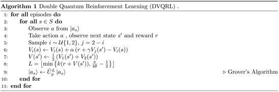
The algorithm for DVQRL can be seen in Algorithm 1.

2.2. Multiple Quantum Reinforcement Learning (MVQRL)

Multiple Quantum Reinforcement Learning (MVQRL) is similar to Double Quantum Reinforcement Learning, but allows for N action value functions instead of only 2. Similar to Multiple Q-learning, the effect of increasing the number of functions is an improvement in learning in stochastic environments. The estimated value of each state is stored in the functions $V_1\left(s\right)\mathrm{,}{V}_2\left(s\right)\mathrm{,}\cdots \mathrm{,}{V}_N\left(s\right)$ . The value functions are updated at each step according to

$V_i\left(s\right)\leftarrow V_i\left(s\right)+\alpha \left(r+\frac{\gamma }{N-1}{\displaystyle \underset{j=1,j\ne i}{\overset{N}{\sum }}}{V}_j\left(s^{\prime }\right)-V_i\left(s\right)\right),$

where $i\sim \mathcal{U}\left\{\mathrm{1,}N\right\}$ . The algorithm for Multiple VQRL may be seen in Algorithm 2.

2.3. Quantum Q-Learning (QQRL)

The idea of Quantum Reinforcement Learning may also be adapted to utilize an action value function instead of a value function. The advantage of this is that the action value function holds more specific information than the value function, potentially leading to faster convergence. In this context, an algorithm is considered to have converged if subsequent updates do not change the policy. Quantum Q Reinforcement Learning (QQRL), which adapts VQRL, has an action value function that replaces the value function in VQRL. This action value function is used to compute the expected value of the next state according to

$V_{s^{\prime }}=\underset{a^{\prime }}{\max }Q\left(s^{\prime }\mathrm{,}{a}^{\prime }\right)\mathrm{,}$

where $Q\left(s\mathrm{,}a\right)$ is the expected value of taking action a from state s, and $V_{s^{\prime }}$ is the expected value of the agent being in state $s^{\prime }$ under the current policy. Like VQRL, in QQRL the policy $|a_s\rangle$ is updated according to

$|a_s\left(t+1\right)\rangle ={\hat{U}}_g^L|a_s\left(t\right)\rangle \mathrm{.}$

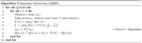
The full algorithm describing QQRL is shown in Algorithm 3.

2.4. Double Quantum Q-Learning (DQQRL)

Similar to VQRL and Double Q-learning, QQRL may be doubled to use two different action value functions, $Q_1\left(s\mathrm{,}a\right)$ and $Q_2\left(s\mathrm{,}a\right)$ . This algorithm is described in (Algorithm 4). At each time step, only one function in the algorithm is updated at a time; this is done by sampling $i\sim \mathcal{U}\left\{\mathrm{1,2}\right\}$ , $j=2-i$ , and applying the update

$Q_i\left(s\mathrm{,}a\right)\leftarrow Q_i\left(s\mathrm{,}a\right)+\alpha \left(r+\gamma Q_j\left(s^{\prime }\mathrm{,}\underset{a^{\prime }}{\arg \max }{Q}_i\left(s^{\prime }\mathrm{,}{a}^{\prime }\right)\right)-Q_i\left(s\mathrm{,}a\right)\right)\mathrm{.}$

When computing L to determine the number of Grover iterations to be performed on the policy, $V\left(s\right)$ is computed according to

$V\left(s\right)=\underset{a}{\max }\frac{1}{2}\left(Q_1\left(s,a\right)+Q_2\left(s,a\right)\right).$

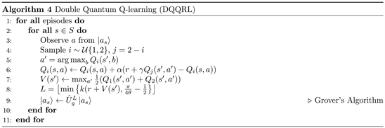
The policy is then updated in the same way as in QQRL.

2.5. Multiple Quantum Q-Learning (MQQRL)

QQRL may also be extended to have any number of action value functions; this is done in a similar way to Multiple Q-learning and MVQRL. The algorithm for Multiple Quantum Q-learning (MQQRL) may be seen in (Algorithm 5). At each time step, a single function is chosen to be updated; this is done by sampling $i\sim \mathcal{U}\left\{\mathrm{1,}N\right\}$ updated according to

$Q_i\left(s,a\right)\leftarrow Q_i\left(s,a\right)+\alpha \left(r+\frac{\gamma }{N-1}{\displaystyle \underset{j=1,j\ne i}{\overset{N}{\sum }}}{Q}_j\left(s^{\prime },b\right)-Q_i\left(s,a\right)\right),$

where $b=\arg {\max }_{a^{\prime }}{Q}_i\left(s^{\prime },a^{\prime }\right)$ . In order to compute the number of Grover iterations, L, $V\left(s\right)$ is computed according to

$V\left(s\right)=\underset{a}{\max }\frac{1}{N}{\displaystyle \underset{i=1}{\overset{N}{\sum }}}{Q}_i\left(s,a\right).$

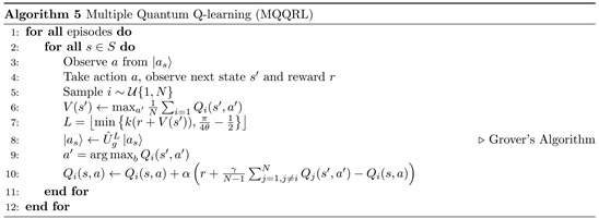
The probability amplitudes of the policy are then updated in the same way as in QQRL.

3. Results

3.1. Test Environment and Optimal Paths

The grid environment used to test the algorithms can be seen in Figure 1. At each time step, the agent may move between adjacent states through the actions up, down, left, and right. The two optimal paths through the environment are shown in Figure 2. This is the environment used by Brown [26] , and is similar to grid environments used in recent studies of quantum computing-based reinforcement learning [23] [24] . While the state and action spaces of these environments are small, they simplify the process of analysis while the field is still in early stages of development. Furthermore, these small state and action spaces lend themselves to implementation on current quantum computing hardware; for example, Sriarunothai, et al. [20] were able to implement an ion-trap reinforcement learning agent with only 2 qubits as a proof of concept.

In order to denote paths through the environment, an action sequence is used. This is a string of action numbers; the mapping from number to action may be seen in Table 1. For example, a path might be denoted by “31210”; this represents the movements right, down, left, down, and up, in sequence. Note that an action may not change the state; if the agent is in its initial position and follows the path “000”, it will remain in the same position.

The “pit” and the “goal” are terminal states; that is, when the agent enters these states, the episode is finished. When the agent enters the “pit”, it receives a reward of $r=-10$ , and when it enters the “goal”, it receives a reward of $r=+10$ . When it enters any of the other states, it receives a reward with mean $\bar{r}=-1$ and standard deviation $\sigma$ . In a deterministic environment, $\sigma =0$ ; in a stochastic environment, $\sigma \ne 0$ , and the agent receives the rewards $-1+\sigma$ and $-1-\sigma$ with equal probability.

Figure 1. Environment used to test each algorithm. A represents the starting location of the agent in the environment, P represents the pit, where the agent receives a large negative reward, W represents the wall, which is a disallowed state, and G represents the goal, where the agent receives a large positive reward. At each time step, the agent receives a small negative reward so that the optimal policy is the shortest path through the environment from the initial state to the goal.

Figure 2. Optimal and sub-optimal paths through the environment. The optimal path (left) corresponds to an action sequence of 33111, while the sub-optimal path (right) corresponds to an action sequence of 31311. Although both paths have the same number of steps, the sub-optimal path is closer to the pit; for stochastic policies, this means that there is an increased probability that the agent will take an action that moves into this state.

Table 1. Numerical labels of each action. A string of these actions such as 32132 indicates a path through the environment.

Due to the stochastic nature of the quantum algorithms, the results for convergence were averaged over multiple runs for each experiment. The number of repeated runs was different for each experiment; these are given in the text and figure captions. In each repeated run, the only difference between the algorithms was the seed value for random number generation. In other words, the position of each feature was the same as in Figure 1 in every run.

3.2. Convergence Properties

One of the most important differences between the single value function algorithms (Q-learning, VQRL, and QQRL) with the corresponding multiple value function algorithms (Multiple Q-learning, MVQRL, and MQQRL) is an increase in stability with the addition of value functions. This is most clearly seen in Figure 3, which plots the breakdown learning rate against the number of value functions for algorithm. As the number of functions increases, all three algorithms become more robust, allowing higher learning rates to be used. One reason for this is that each function is constructed using only a fraction of the overall experiences. Combining these functions then results in an estimate of the value or the action value which is less sensitive than when only a single function is used.

The breakdown learning rate was defined in the same manner as above for the single value function algorithms; in other words, the value of $\alpha$ past which $N>1000$ . This was computed for Multiple Q-learning, MVQRL, and MQQRL for each value of $N\in \left[1,10\right]$ and is shown in Figure 3. From this, it can be seen that for each of the three algorithms, increasing the number of value functions (either $Q\left(s\mathrm{,}a\right)$ or $V\left(s\right)$ ) increases the learning rate at which the algorithms break down; in other words, additional value functions increase the stability of the policy.

Another feature of Figure 3 to note is that MQQRL consistently has a higher breakdown learning rate than Multiple Q-learning and MVQRL. This indicates that, for the same N, MQQRL is more robust to a higher learning rate. One advantage of this is that a higher learning rate may be set with MQQRL than MVQRL, which generally increases the speed of learning. Furthermore, both Multiple Q-learning and MQQRL have higher breakdown learning rates for $N>1$ , which indicates that $Q\left(s\mathrm{,}a\right)$ is a more robust against higher learning rates than $V\left(s\right)$ .

Similar to the learning rate, the parameter k also has a significant effect on the convergence of the quantum algorithms; effectively, it determines how quickly the policy changes. A larger k results in a faster change in the policy, which generally means that the learning rate of the algorithm increases. This may be seen in Figure 4.

The relationship between k and the speed of convergence of VQRL and QQRL is interesting because, above a certain threshold, the number of episodes until convergence remains steady at around 12.5. This indicates that the algorithms are not sensitive to the particular value of k, given that it is sufficiently high, which suggests that a reasonable strategy for the selection of a particular k value may be to increase the value until the number of iterations to convergence does not change anymore.

3.3. Branching Ratios of Optimal and Sub-Optimal Paths

While the speed of convergence is an important characteristic when comparing any computer algorithms, it is also important to consider the quality of the policies the algorithms generate and the paths through the environment that they produce. An interesting comparison between Q-learning, VQRL and QQRL is the relative path distribution between each of the algorithms. Ideally, each of the algorithms will converge over time to the optimal path, which is often the shortest path. The branching ratio, which is the fraction of times that the algorithm converged to a certain path, can be seen as a function of episode number in Figure 5.

Figure 3. Breakdown learning rate as function of the number of $Q\left(s\mathrm{,}a\right)$ functions. The breakdown learning rate is the minimum value of $\alpha$ where the algorithm fails to find the goal. Note that $N=1$ corresponds to Q-learning, QQRL, and VQRL, and that $N=2$ corresponds to Double Q-learning, DQQRL, and DVQRL.

Figure 4. Iterations to convergence as a function of k in a deterministic environment. The results were averaged over 100,000 runs. For this experiment, $\alpha =0.05$ .

Figure 5. Branching ratio of Q-learning, VQRL, and QQRL. The optimal path 33111 and the suboptimal path 31311 are shown in Figure 2. For this experiment, $\alpha =0.05$ . The results were averaged over 1000 runs.

While Q-learning converges slower than VQRL and QQRL, over time it converges to the optimal path instead of the sub-optimal path. However, when VQRL and QQRL converge to the sub-optimal path, their policies have become essentially deterministic; consequently, there is little difference between the optimal path and the sub-optimal path as both have are the same length. The only reason why the sub-optimal path is less ideal than the optimal one is because it is closer to the “pit”, so an agent with a stochastic policy has a higher probability of entering the “pit”.

The reason for why the policies of VQRL and QQRL become deterministic over time may be attributed to repeated applications of Grover’s algorithm to the policies. In these algorithms, Grover iterations have the tendency to increase the probability of actions with higher expected returns and decrease actions with lower ones. As the value functions of these algorithms converge, repeated Grover iterations tend to increase the probability of the most favorable action―the action with the highest expected return―and decrease the probability of all of the other actions. In the limit, the probability of the action with the maximum expected return approaches 1, and the probabilities of all other actions approach 0. In effect, the probability becomes deterministic in the limit.

While it is clear in Figure 5 that VQRL and QQRL converge much faster than Q-learning, it is also apparent that Q-learning tends to converge to the optimal path over time, while the quantum algorithms converge to a distribution between the optimal and sub-optimal paths. This highlights one trade off between the quantum algorithms and their classical counterparts: while the quantum algorithms converge much faster to a less optimal path distribution, Q-learning eventually converges to the optimal path.

3.4. Comparison of Value Functions for VQRL, QQRL, and Q-Learning

An important difference between Q-learning, VQRL, and QQRL is the estimate of the value of each of the states; these are shown in Figure 6 for the initial state

Figure 6. Expected value of initial state for Q-learning, VQRL, and QQRL. For VQRL, $V\left(s\right)$ is shown, but for QQRL and Q-learning $V_{\max }\left(s\right)=\arg {\max }_{a}Q\left(s,a\right)$ is shown for comparison. The true value ( $V\left(s\right)=3.122$ ) is also shown for comparison. For this experiment, $\alpha =0.05$ ; the results were averaged over 1000 runs.

of the agent as a function of the number of episodes. In the experiment shown, VQRL and QQRL converge much faster to the expected value of the state. As the stability of the value function is highly related to the stability of the policy, this indicates that the policies of VQRL and QQRL converge much quicker than Q-learning. An interesting distinction between VQRL and QQRL is that VQRL converges to a much higher value than QQRL. While the cause of this is uncertain, it is likely related to the path distribution that the algorithm converges to (see Figure 5).

In addition to the maximum value of the state, Q-learning and QQRL exhibit further differences in the value of each action for the state. This is shown in Figure 7 for the initial state. An interesting observation is that for the first 100 episodes, $Q\left(s\mathrm{,}a\right)$ for Q-learning and QQRL follow the same downward trend for each a. After episode 100, however, the values diverge; QQRL converges much faster than Q-learning, which does not converge in the first 1000 episodes.

3.5. Comparison of Value Functions for Double Q-Learning, DVQRL, and DQQRL

One of the effects of doubling the value functions of reinforcement learning algorithms is that the expected value of each state is different for each state. Generally, this difference is an underestimate in comparison with the estimate of the value in the single function algorithm; this may be observed in Figure 8. However, despite this initial underestimate at any given episode, the shape of the double function algorithms generally follows the shape of the single function algorithms, but at a slower rate.

3.6. Comparison of Value Functions for Multiple Q-Learning, MVQRL, and MQQRL

Like Double Q-learning, DVQRL, and DQQRL, Multiple Q-learning, MQVRL, and MQQRL also exhibit underestimation of $Q\left(s\mathrm{,}a\right)$ and $V\left(s\mathrm{,}a\right)$ for the single versions of the algorithms (Q-learning, VQRL, and QQRL). This is shown for $N=3,6,10$ in Figure 9. An interesting feature of MQQRL graph is that, as the number of $Q\left(s\mathrm{,}a\right)$ functions increases, the initial amount of underestimate of the value exhibited by MQQRL increases. Furthermore, as may be seen for $N=3$ and implied for $N=6$ , the value which MQQRL converges to is greater than QQRL. Neither of these behaviors are exhibited by MVQRL, which essentially has the same behavior as VQRL but at a slower rate.

Figure 7. Comparison of $Q\left(s\mathrm{,}a\right)$ for Q-learning and QQRL for each action. Clockwise from top left, the actions shown are Up, Down, Left, and Right. For this experiment, $\alpha =0.05$ ; the results were averaged over 1000 runs.

Figure 8. Comparison of $V\left(s\right)$ between single function algorithms (Q-learning, VQRL, QQRL) with corresponding double function algorithms (Double Q-learning, DVQRL, DQQRL) for the initial state. The true value ( $V\left(s\right)=3.122$ ) is shown for comparison. For Q-learning, Double Q-learning, QQRL, and DQQRL, $V\left(s\right)$ was computed according to $V_{\max }\left(s\right)={\max }_{a}Q\left(s,a\right)$ .

Figure 9. Comparison of $V\left(s\right)$ between single function algorithms (Q-learning, VQRL, QQRL) with corresponding multiple function algorithms (Multiple Q-learning, MVQRL, MQQRL) for the initial state. The values of $N=3$ , $N=6$ , and $N=10$ were chosen to sample the effect of increasing N. For Q-learning, Multiple Q-learning, QQRL, and MQQRL, $V\left(s\right)$ was computed according to $V_{\max }\left(s\right)={\max }_{a}Q\left(s,a\right)$ . The top row shows the case where $N=3$ , the middle row $N=6$ , and the bottom row $N=10$ . In each row, the first graph compares Q-learning with Multiple Q-learning, the second graph compares VQRL with MVQRL, and the third graph compares QQRL with MQQRL. The true value ( $V\left(s\right)=3.122$ ) is shown for comparison.

3.7. Comparison of CPU Time

An important metric when comparing reinforcement learning algorithms is the relative computational efficiency of each. The average amount of computation time per episode for each algorithm implemented is shown in Table 2, in units of μs, and the average computation time to reach convergence is shown in Table 3 in units of μs. It may be observed that the classical algorithms have higher efficiency per episode in Table 2; however, Table 3 shows that the quantum algorithms show much better performance overall, converging in significantly less time because they require less iterations to converge. The time measurements were made on an Intel i5-3210M processor with 8 GB of DDR3 RAM. The algorithms were implemented with multiple threads in C++ and compiled with GCC 6.3.1-1; however, CPU times were normalized to give the required CPU time in a single thread.

Table 2. CPU time per episode (μs/episode) for each algorithm.

Table 3. CPU time to reach convergence (μs) for each algorithm.

Another interesting feature highlighted by Table 2 and Table 3 is the relationship between the CPU time and the number of $V\left(s\right)$ or $Q\left(s\mathrm{,}a\right)$ functions in each algorithm. For MVQRL and Multiple Q-learning, there is a weak relationship between the CPU time per episode and the number of $V\left(s\right)$ or $Q\left(s\mathrm{,}a\right)$ functions. However, the CPU time per episode for QQRL shows a strong dependence on the number of $Q\left(s\mathrm{,}a\right)$ functions. MQQRL also exhibits a strong relationship between the number of $Q\left(s\mathrm{,}a\right)$ functions and the CPU time required to reach convergence, as does Multiple Q-learning, but MVQRL does not. This is an interesting result, indicating that there is little computational penalty for increasing the number of $V\left(s\right)$ functions in MVQRL, providing the benefits of multiple functions with only a marginal increase in CPU usage.

As may be seen in Table 2, MQQRL requires significantly more CPU than Multiple Q-learning or MVQRL for large values of N. There are multiple possible causes of this; first, MQQRL requires the calculation of

$V_{s^{\prime }}={\max }_{a^{\prime }}\frac{1}{N}{\displaystyle {\sum }_{i=1}^N}{Q}_i\left(s^{\prime },a^{\prime }\right)$ on every iteration, scaling linearly with the number

of $Q\left(s\mathrm{,}a\right)$ functions. Additionally, the memory fragmentation of the particular implementation may play largely into the additional CPU time; each $Q\left(s\mathrm{,}a\right)$ was stored as vector of rows, where each row was stored separately. On the other hand, in MVQRL each $V\left(s\right)$ function was stored as a vector, meaning that the entire function was stored contiguously in memory. Thus, it is likely that MQQRL causes significantly more cache misses than MVQRL in the current implementation, increasing the CPU time for the algorithm. A more robust solution might store the entire $Q\left(s\mathrm{,}a\right)$ function in a contiguous array to reduce cache misses.

However, despite the fact that MQQRL requires more CPU time per episode than MVQRL, it is balanced to a certain degree by the fact that MQQRL requires fewer iterations to converge. However, there are many situations in which fewer iterations is more desirable than overall computation time, and in these scenarios MQQRL may be a better choice than MVQRL. An example scenario might be one where the physical cost of exploration is high but computational expense is low, in which case it may be advantageous to decrease the number of iterations required to converge and use a more powerful computer.

The increase in CPU time to reach convergence with N for Multiple Q-learning may be attributed to an increase in the number of episodes required to reach convergence, as the CPU time per episode is effectively constant. However, for MQQRL the increase in CPU to reach convergence may be attributed to both an increase in the number of episodes as well as an increase in the CPU time per episode. For all N, however, MVQRL and MQQRL completed in less CPU time than Multiple Q-learning, meaning that the benefits of the Quantum algorithms over the classical ones may be realized with less computational expense, not more.

3.8. Summary of Results

The results in Section 3.2 demonstrate that QQRL reaches convergence in fewer episodes than VQRL. QQRL and VQRL only differ in how the value of the current state is stored; that is, QQRL uses $Q\left(s\mathrm{,}a\right)$ while VQRL only uses $V\left(s\right)$ . Likely, the reason for such improvement in convergence speed is due to the extra precision provided by $Q\left(s\mathrm{,}a\right)$ when computing the value of a certain action and then choosing the best action; in contrast, $V\left(s\right)$ is the expectation of the value of all possible actions, and as a consequence is much less precise. The extra precision is especially important when updating the policy in QQRL as it uses ${\max }_{a}Q\left(s\mathrm{,}a\right)$ to compute the number of Grover iterations to perform.

Another important observation is that the quantum algorithms, VQRL, QQRL, MVQRL, and MQQRL, have much faster convergence than their classical counterparts, Q-learning and Multiple Q-learning. As discussed by Dong, et al. [25] , this is likely the quantum algorithms strike a better balance between exploration and exploitation in the way the policies are updated, at least as compared to the classical algorithms. This is because the quantum algorithms store the policy as a superposition of all possible algorithms, and use Grover’s algorithm to increase the probability of taking an action. Furthermore, because the quantum algorithms are probabilistic in nature, they are more robust in environments with a stochastic reward signal.

Finally, it was found that adding extra $V\left(s\right)$ and $Q\left(s\mathrm{,}a\right)$ functions improved the learning in a stochastic environment. In other words, when the reward was drawn from some distribution, MVQRL and MQQRL exhibited better performance than VQRL and QQRL, respectively, in the same way that Multiple Q-learning exhibited better performance than Q-learning [11] . This is because

each $V_i\left(s\right)$ or $Q_i\left(s\mathrm{,}a\right)$ function is constructed using only $\frac{1}{N}$ of the total

number of experiences, and the variations among the function are reduced when computing the average $V\left(s\right)$ or $Q\left(s\mathrm{,}a\right)$ .

4. Discussion

4.1. Convergence of Quantum and Classical Algorithms

One comparison which may be drawn between the quantum and classical algorithms is the number of episodes to convergence. Generally, it was observed that the value functions $V\left(s\right)$ and $Q\left(s\mathrm{,}a\right)$ in VQRL and QQRL, respectively, converge much faster than the $Q\left(s\mathrm{,}a\right)$ in Q-learning. This result leads to significantly faster convergence times for the same learning rate; for smaller learning rates, the quantum algorithms converge about 10 times faster. Additionally, the quantum algorithms were found to be less CPU intensive than their classical counterparts for a given number of $Q\left(s\mathrm{,}a\right)$ or $V\left(s\right)$ functions, meaning that although the quantum algorithms presented in this paper were not realized on a quantum computer, their use on a classical computer can still provide benefits over the classical algorithms.

A particular feature of QQRL is that it has a higher breakdown learning rate than either Q-learning or VQRL; this generalizes to Multiple Q-learning, MQVRL, and MQQRL. QQRL not only converges faster than Q-learning for a certain learning rate, but also allows for higher learning rates than Q-learning does. This is an interesting phenomenon which indicates that QQRL gives faster convergence in general than Q-learning.

4.2. Comparison of QQRL with VQRL

One of the main differences between VQRL and QQRL is the convergent path distribution for each algorithm (see Figure 5). While QQRL converges in 25% fewer episodes than VQRL, it converges to a path distribution that equally weights the optimal and sub-optimal paths. However, both paths are the same length; the sub-optimal path is only considered such because an agent with a stochastic policy is more likely to move into the “pit” (and receive a large negative reward). Thus, the fact that QQRL converges to an equal path distribution indicates that the policy is highly deterministic, in which case there is no advantage of one path over the other.

4.3. Final Remarks

This paper introduced the novel algorithm called Quantum Q-learning (QQRL), which replaced the value function $V\left(s\right)$ in Quantum Reinforcement learning (VQRL) with the action-value function $Q\left(s\mathrm{,}a\right)$ . It was found that QQRL converged faster than VQRL, due to the added precision of $Q\left(s\mathrm{,}a\right)$ which more efficiently incorporates updates than $V\left(s\right)$ . It was also found that QQRL converged much faster than classical Q-learning. Furthermore, QQRL was found to be more robust to higher learning rates than VQRL, allowing even faster convergence.

This paper also introduced the algorithms Multiple VQRL (MVQRL) and Multiple QQRL (MQQRL) by introducing multiple estimates of $V\left(s\right)$ and $Q\left(s\mathrm{,}a\right)$ into VQRL and QQRL, respectively. These algorithms are shown to be more tolerant of higher learning rates, and are found to more effectively handle stochastic rewards, with the effect increasing with the number of value functions. This is similar to the fashion in which additional functions in Multiple Q-learning tended to improve the stability. Each additional function decreases the number of experiences used to train each individual function. Averaging over these then produces a better estimate of the value or action value than each individual function.

The results of this paper demonstrate that a qubit-based policy works well with action-value ( $Q\left(s\mathrm{,}a\right)$ ) reinforcement learning techniques, even when the reward signal is noisy. This is a significant step toward more complex quantum reinforcement learning algorithms, especially those based on the classical concepts of value-based reinforcement learning. The algorithms discussed in this paper demonstrate the viability of research in this direction.

Finally, it was found that CPU time required the quantum algorithms to converge was significantly less that the amount of time required for the corresponding classical algorithms with the same number of $Q\left(s\mathrm{,}a\right)$ or $V\left(s\right)$ functions. This is an interesting result, as it indicates that utilization of the quantum algorithms on a classical computer yields an improvement in computational speed over the classical algorithms. Furthermore, this means that more $V\left(s\right)$ or $Q\left(s\mathrm{,}a\right)$ functions may be used, improving the ability of the quantum algorithms to handle noisy signals.

Acknowledgements

We would like to thank Houghton College for providing financial support for this study. We would also like to thank the anonymous reviewer for their helpful comments.

Conflicts of Interest

The authors declare no conflicts of interest.

References

[1]	Brown, B. (2015) Q-Learning with Neural Networks.
[2]	Dong, D., Chen, C., Li, H. and Tarn, T.-J. (2008) Quantum Reinforcement Learning. IEEE Transactions on Systems, Man, and Cybernetics, Part B (Cybernetics), 38, 1207-1220. https://doi.org/10.1109/TSMCB.2008.925743
[3]	Duryea, E., Ganger, M. and Hu, W. (2016) Exploring Deep Reinforcement Learning with Multi Q-Learning. Intelligent Control and Automation, 7, 129. https://doi.org/10.4236/ica.2016.74012
[4]	Grover, L.K. (1996) A Fast Quantum Mechanical Algorithm for Database Search. Proceedings of the Twenty-Eighth Annual ACM Symposium on Theory of Computing, Philadelphia, 22-24 May 1996, 212-219. https://doi.org/10.1145/237814.237866
[5]	Hasselt, H.V. (2010) Double Q-Learning. Advances in Neural Information Processing Systems, 23, 2613-2621.
[6]	Kober, J., Bagnell, J.A. and Peters, J. (2013) Reinforcement Learning in Robotics: A Survey. The International Journal of Robotics Research, 32, 1238-1274. https://doi.org/10.1177/0278364913495721
[7]	Lee, J.W. (2001) Stock Price Prediction Using Reinforcement Learning. 2001 IEEE International Symposium on Industrial Electronics Proceedings, Pusan, 12-16 June 2001, 690-695.
[8]	Mnih, V., Kavukcuoglu, K., Silver, D., Graves, A., Antonoglou, I., Wierstra, D. and Riedmiller, M. (2013) Playing Atari with Deep Reinforcement Learning. arXiv preprint arXiv:1312.5602.
[9]	Shor, P.W. (1994) Algorithms for Quantum Computation: Discrete Logarithms and Factoring. Proceedings 35th Annual Symposium on Foundations of Computer Science, Santa Fe, 20-22 November 1994, 124-134. https://doi.org/10.1109/SFCS.1994.365700
[10]	Silver, D., Huang, A., Maddison, C.J., Guez, A., Sifre, L., Van Den Driessche, G., Schrittwieser, J., Antonoglou, I., Panneershelvam, V., Lanctot, M., et al. (2016) Mastering the Game of Go with Deep Neural Networks and Tree Search. Nature, 529, 484-489. https://doi.org/10.1038/nature16961
[11]	Sutton, R.S and Barto, A.G. (1998) Reinforcement Learning: An Introduction, Volume 1. MIT Press, Cambridge.
[12]	Tromp, J. (2016) Number of legal Go Positions.
[13]	Van Hasselt, H., Guez, A. and Silver, D. (2016) Deep Reinforcement Learning with Double Q-Learning. AAAI, 2094-2100.
[14]	IBM (2017) IBM Builds Its Most Powerful Universal Quantum Computing Processors.
[15]	Biamonte, J., Wittek, P., Pancotti, N., Rebentrost, P., Wiebe, N. and Lloyd, S. (2017) Quantum Machine Learning. Nature, 549, 195. https://doi.org/10.1038/nature23474
[16]	Cárdenas-López, F.A., Lamata, L., Retamal, J.C. and Solano, E. (2017) Generalized Quantum Reinforcement Learning with Quantum Technologies. PLoS ONE, 13, e0200455. arXiv:1709.07848
[17]	Cao, Y., Guerreschi, G.G. and Aspuru-Guzik, A. (2017) Quantum Neuron: An Elementary Building Block for Machine Learning on Quantum Computers. arXiv:1711.11240
[18]	Crawford, D., Levit, A., Ghadermarzy, N., Oberoi, J.S. and Ronagh, P. (2016) Reinforcement Learning Using Quantum Boltzmann Machines. arXiv:1612.05695
[19]	Hu, W. (2018) Empirical Analysis of Decision Making of an AI Agent on IBM 5Q Quantum Computer. Natural Science, 10, 45. https://doi.org/10.4236/ns.2018.101004
[20]	Hu, W. (2018) Towards a Real Quantum Neuron. Natural Science, 10, 99. https://doi.org/10.4236/ns.2018.103011
[21]	Levit, A., Crawford, D., Ghadermarzy, N., Oberoi, J.S., Zahedinejad, E. and Ronagh, P. (2017) Free Energy-Based Reinforcement Learning Using a Quantum Processor. arXiv:1706.00074
[22]	Nielsen, M.A. and Chuang, I.L. (2011) Quantum Computation and Quantum Information: 10th Anniversary Edition. 10th Edition, Cambridge University Press, New York.
[23]	Sallans, B. and Hinton, G.E. (2004) Reinforcement Learning with Factored States and Actions. Journal of Machine Learning Research, 5, 1063-1088.
[24]	Sriarunothai, T., Wolk, S., Giri, G.S., Fries, N., Dunjko, V., Briegel, H.J. and Wunderlich, C. (2017) Speeding-Up the Decision Making of a Learning Agent Using an Ion Trap Quantum Processor. arXiv:1709.01366
[25]	Watkins, C.J.C.H. (1989) Learning from Delayed Rewards. PhD Thesis, University of Cambridge, Cambridge.
[26]	Williams, R.J. (1992) Simple Statistical Gradient-Following Algorithms for Connectionist Reinforcement Learning. Machine Learning, 8, 229-256. https://doi.org/10.1007/BF00992696