Quantification of Reservoir Fluid Prediction Uncertainty Using AVO Fluid Inversion (AFI) ()
1. Introduction
In the late 1920s, the seismic reflection technique became a key tool for the oil industry, illuminating shapes of subsurface structures and indicating possible drilling targets. This has developed into a multibillion dollar business that is still primarily concerned with structural interpretation. But advances in data acquisition, processing and interpreting now, make it possible to use seismic traces to reveal more than just subsurface reflector shape and position.
Changes in the character of seismic pulses returning from a subsurface reflector can now be interpreted to ascertain the depositional history of a basin, the rock type in a layer, and even the nature of the pore fluid. This last refinement, pore fluid identification, is the ultimate goal of AVO analysis. Amplitude variation with offset, AVO has become an essential tool in the petroleum industry for hydrocarbon detection [1] . Among the various seismic technique for hydrocarbon detection and monitoring in the subsurface, amplitude variation with offset (AVO) methods appears to be quite promising. The AVO is measured in the primary P-wave reflections, which are the strongest and freest from contamination, and at the same time, they contain the information about the S-wave reflectivity.
AVO is the generic name for a wide class of advanced methods for analyzing the amplitude of pre-stack seismic data, aimed at characterizing the fluid content or the lithology of a possible reservoir [2] [3] .
The acronym AVO stands for Amplitude Versus Offset (analysis) and the name itself suggests that we are operating in the CDP (Common Depth Point) domain in which seismic traces recorded with variable source-receiver distances are grouped according to common reference points in the subsurface. This collection of traces is referred to as a common midpoint (CMP) gather. In conventional seismic processing, in which the goal is to create a seismic section for structural or stratigraphic interpretation, traces in a gather are stacked-summed to produce a single average traces [4] .
The AVO method enables recovery of some of the information lost by the stack technique, leading to an economic and robust (in a statistical sense) increase in the quality of the seismic section, when dealing with difficult but conventional interpretative situations.
The physical principle on which the AVO analysis is actually based is the variation in the reflected energy at each seismic horizon as the incidence angle of the wave-front varies. This variability is mathematically described by rather complex relationships called the Zoeppritz equations and is a primary function of the elastic parameters of the two rocks which limit the interface: velocity of the P-waves, density and Poisson’s coefficient (or the almost directly related Vp/Vs ratio). Because of the nonlinearity of the Zoeppritz equations, several approximations have been generated, such as those presented by [5] [6] . Different lithological compositions and different fluid contents translate into variations of the elastic parameters of the rocks. This accounts for the variability of the acoustic behavior at the reflector as the offset of the seismic pre-stack data varies: these variations are the subject of the AVO analysis.
Quantitative AVO analysis is done on common-midpoint-gathers or Ostrander gathers [2] . At each time sample amplitude values from every offset in the gather are curve-fit to a simplified, linear AVO relationship. By imposing a best-fit straight line to a plot of amplitude versus some function of the angle of incidence we derive two important AVO attributes namely; the slope (G) and intercept (I) of a straight line, which describes how the amplitude behaves with angle of incidence as shown in Figure 1.
The main limitation of the AVO analysis method is always the relatively poor link between the theoretical models (Pre-stack synthetic seismograms) and the AVO measurements from real seismic data.
![]()
Figure 1. Derivation of Gradient (G) and Intercept (I) from Ostrander gathers.
AVO Fluid Inversion methodology is an answer to this need. This is still based on the well known AVO technology of exploiting seismic pre-stack data information. But special emphasis is given here to get a quantitative probability estimate of the possible reservoir fluids. This is achieved through the development of a stochastic AVO model and an inversion to probability of different fluids using the Bayesian approach.
The overall aim of this study is to use the AVO Fluid Inversion (AFI) technique to assess for fluids at the target levels of the study area. This method is expected to provide a quantitative probability estimation of different fluids occurrence in the target reservoirs.
2. Location of the Study Area
The DW_OPL_X is located in the Southern Ultra Deepwater Province of the Nigeria Offshore where water depth varies from 1900 m to 2960 m (Figure 2).
The most striking geological feature in the Niger Delta Basin is a huge prograding Deltaic complex whose shoreline, since the Cretaceous, gradually moved toward SW over a distance of some hundreds of km [7] .
In Deltaic systems, simple facies distribution models are based on subdivision in shelfal, slope and basinal depositional settings. This simple model is complicated by a syn-depositional tectonics activity affecting both the sediment dispersal pattern and sand accumulation (Figure 3).
![]()
Figure 3. Arbitrary seismic line through existing wells.
3. Materials and Methods
The following data was used in the study:
(i) Seismic Data
The seismic input data for the study consist on the Narrow and Wide Partial Angle Stacks (5 - 15 and 25 - 40 Incidence Angle Degrees) covering the whole block. Processing was carried out with an Amplitude Preserving processing sequence including Kirchhoff PSTM and 4th order Anisotropic Move-out. The data was in SEG-Y format.
(ii) Well Data
Wireline logs (In LAS format)
・ P-wave sonic (DT)
・ Density (RHOB)
・ S-wave sonic (DTS)
・ Lithologic log (Gamma Ray)
・ Resistivity
(iii) The softwares used in this study are:
・ Openworks softwares, A proprietary software Fluid Inversion, Microsoft Excel and Word.
The methodology adopted for the study involves four steps as shown below:
1. A horizon interpretation and amplitude (both Near and Far) picking of the expected reservoir sand top interfaces (Figure 4(a) and Figure 4(b)).
2. An apriori AVO stochastic model, which brings into the prediction engine the expectations of the change of AVO parameters I and G (intercept and gradient) with the acceptable variation of the petro-physical parameters of the reservoirs and the encasing shale (porosity, moduli of rocks and fluids, etc.) (Figure 5 and Figure 6).
3. Calibration (re-scaling) of picked Near and Far amplitudes to the model and validation at well locations (Figure 7 and Figure 8).
4. Final computation of fluid probability maps (gas, oil, brine) is then carried out through a Bayesian inversion approach (computation of posterior probability of I-G real data pairs to belong to each of the modelled saturating fluids) (Figures 9-12).
4. Fluid Probability Estimation
In probabilistic terms, we are considering three classes of fluid (brine, oil, gas) each described by a set of samples Sbrine, Soil, Sgas. We are interested in estimating the posterior probability that a single (I, G) point from real AVO measurement belongs to one specific class.
This is achieved by fitting a conditional probability density function to each set of data point in the model:
Sbrine p(I, G|brine) Sgas p(I, G|gas) Soil p(I, G|oil)
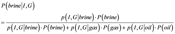
And then computing posterior probabilities P(brine|I, G), P(gas|I, G), P(oil|I, G) by means of the Bayes rule:
Interpretation Results of the Target Objects
![]()
![]()
Figure 4. (a) Interpreted horizon on near seismic volume; (b) Interpreted horizon on far seismic volume.
![]()
Figure 5. Nigeria deepwater AFI model-gas probability.
![]()
Figure 6. Nigeria deepwater AFI model-Oil probability.
![]()
Figure 7. AFI calibration at dou-1 well location.
![]()
Figure 8. AFI calibration at Emein-1 well location.
 (1)
(1)
where P(brine), P(gas), P(oil) are a priori probabilities (if an uniform prior probability is assumed, as we do, they are all equal to 1/3). To get the remaining posterior probabilities, simply replace brine with oil or gas in the same equation. Currently we do assume a Cauchy distribution for conditional densities:
 (2)
(2)
where d2 is the Mahalanobis distance (a covariance weighted measurement of distance, which is not necessarily isotropic).
In practice, once a stochastic AVO model for the area is available (it should be visualized as a three-dimensional cube of Intercept, Gradient and Burial Depth data points), the inversion of real data AVO measurements into fluid prediction for all the target objects in the active map, basically consists in estimating a “distance” of real I, G couplets from the model clouds at the appropriate depth, and then translating such distances into probabilities (Figure 13 and Figure 14).
Final result of the analysis is typically represented as a set of three maps of probability (brine, oil, gas) as shown in Figures 9-12. Combination maps can also be computed, like “Total HC probability” or “Fluid Indicator”.
5. Conclusion
Overall the “shallow” target levels show positive AVO behavior. Some evidences of a possible gas cap at level L68 are present.
MODEL VALIDATION AND TREND ANALYSIS
![]()
Figure 13. P-wave trend of Nigeria deep water wells.
![]()
Figure 14. Density trend of Nigeria deepwater wells.
As far as the L68 is concerned, some deepening of the sedimentary model is necessary to explain the positive AVO response out of the structure (Figure 9).
However the structural fit within the main structural feature is anyway acceptable.
AVO and DHI response proves almost negative for the deeper levels (L45 and L32). This cannot be explained without accepting a substantial change of the rock petrophysical parameters (especially in the shale).
・ Some absorption effect could also be appealed to trying to explain the amplitude decay with burial depth, but this does not prove to be consistent with the AVO model for the shallower levels (Figure 13).
・ On the other side, a possible transition to an AVO Class II or I at the burial of such “deep” sequence (1600 - 2000 m) is not accounted for by the model in place.
・ Results of the AFI maps show that probability figures for the oil map are moderate to low.