The Theory of Higher-Order Types of Asymptotic Variation for Differentiable Functions. Part I: Higher-Order Regular, Smooth and Rapid Variation

Antonio Granata

Department of Mathematics and Computer Science, University of Calabria, Rende (Cosenza), Italy.

DOI: 10.4236/apm.2016.612063                

Abstract

Motivated by a general theory of finite asymptotic expansions in the real domain for functions f of one real variable, a theory developed in a previous series of papers, we present a detailed survey on the classes of higher-order asymptotically-varying functions where “asymptotically” stands for one of the adverbs “regularly, smoothly, rapidly, exponentially”. For order 1 the theory of regularly-varying functions (with a minimum of regularity such as measurability) is well established and well developed whereas for higher orders involving differentiable functions we encounter different approaches in the literature not linked together, and the cases of rapid or exponential variation, even of order 1, are not systrematically treated. In this semi-expository paper we systematize much scattered matter concerning the pertinent theory of such classes of functions hopefully being of help to those who need these results for various applications. The present Part I contains the higher-order theory for regular, smooth and rapid variation.

Keywords

Higher-Order Regularly-Varying Functions, Higher-Order Rapidly-Varying Functions, Smoothly-Varying Functions, Exponentially-Varying Functions, Asymptotic Functional Equations

1. Introduction

In a previously-published series of papers ( [1] [2] [3] [4] [5] ) we established a general analytic theory of finite asymptotic expansions in the real domain for functions of one real variable sufficiently regular on a deleted neighborhood of a point. The theory is based on the use of a uniquely-determined linear differential operator associated to a given asymptotic scale “”; and the conditions characterizing two sets of expansions obtained from

(1.1)

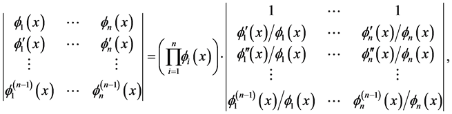
by two special procedures of formal differentiation are expressed via improper integrals involving both the quantity and certain ratios of Wronskians of the. For instance one such condition is

(1.2)

and for practical applications it is quite useful to have some information on the asymptotic behavior of the ratio of Wronskians. For a possible step consists in writing

(1.3)

and then recalling that in various but related contexts the following remarkable asymptotic relations linking the ratios to are found:

(1.4)

or

(1.5)

for different classes of functions. Bourbaki ( [6] ; Chap. V, appendix, pp. V.36-V.40), in the context of Hardy fields, shows their validity for each (some exceptional cases apart) for the classes of functions therein called “of finite order a [respectively, of infinite order] with respect to the function, as” and defined by the property that

(1.6)

Balkema, Geluk and de Haan, ( [7] ; Lemma 9, p. 410), have shown the equivalence of (1.4), written in the form

(1.7)

with the property that the function satisfies

(1.8)

-functions satisfying (1.7)-(1.8) for are called “smoothly varying at with exponent (or index)”: see also Bingham, Goldie and Teugels ( [8] ; p. 44). Another author, Lantsman ( [9] : pp. 96-98), shows the validity of (1.7) for the class of functions such that

(1.9)

such a being said to have a “power order of growth at”.

All these approaches for infinitely-differentiable functions have in common the existence of the following limit

(1.10)

wherein the three contingencies are special cases of the more general classes of functions traditionally labelled as “slowly, regularly or rapidly varying at”. Motivated by the fact that the’s of most asymptotic scales found in applications belong to one of these classes and that the before-mentioned relations for the derivatives have important applications in several fields, we deemed it convenient to systematize the theory of higher-order “types of asymptotic variation” showing the equivalence of various approaches, putting together a large amount of basic properties and highlighting the parallel theory of rapid or exponential variation always cursorily treated. Many proofs have an elementary character left apart: the equivalence of the various approaches based on a remarkable device by Balkema, Geluk and de Haan, and the operations on higher-order varying functions which requires a certain amount of patience. Much time has been spent in giving an abundance of counterexamples to show the necessity of possible restrictive assumptions. A special attention has been paid to listing a variety of asymptotic functional equations satisfied by the functions in the studied classes. Only the general theory has been treated in this semi-expository paper and the applications are restricted to some asymptotic properties of antiderivatives and sums, and to asymptotic expansions of an expression of type. Applications to general asymptotic expansions and differential-functional equations would require a separate treatment. The exposition is on a plain level and an effort has been made to look for the simplest proofs.

- §2 contains a detailed and integrated exposition of basic properties (algebraic, differential and asymptotic) concerning regular and rapid variation in the strong sense. Much, but not all, the material concerning regular variation is standard and the most elementary proofs have been reported. Some facts concerning the index of variation of the first derivative in §2.3 are essential both to give a correct definition of higher-order regular variation and to understand possible restrictions on the indexes.

- In §3 we give an integrated exposition of higher-order regular variation (a concept indirectly encountered in the context, e.g., of Hardy fields) and smooth variation (a concept explicitly present in the literature concerning some applications of regular variation), both traditionally (but not in our approach) referred to -functions. We show the equivalence of different approaches found in the literature reporting a clarified version of a non-trivial characterization by Balkema, Geluk and de Haan trying to highlight the computational ideas in the ingenious proof, somehow hidden in the original exposition.

- In §4 an analogous exposition for higher-order rapid variation is given with several characterizations. To be useful for applications a restriction must be added to the “spontaneous” concept of higher order for this class of functions.

- In §5 there is a discussion about various useful asymptotic functional equations satisfied by the functions in the previously-studied classes.

In part II we exhaustively describe results about algebraic operations on higher-order asymptotically-varying functions and treat concepts related to exponential variation and some of their basic applications.

General notations

-

-

- is absolutely continuous on each compact subinterval of the interval I;

-;

- For we write “” meaning that x runs through the points wherein exists as a finite number;.

- If the usual notation [resp.] means that the improper integral is either convergent or divergent for some T large enough.

- The logarithmic derivative.

- Hardy’s notations:

“” or, equivalently “” stands for ;

“” or, equivalently “” stands for .

- The relation “” which we label as “asymptotic similarity”, means that

(1.11)

- The relation of asymptotic equivalence:

stands for.

- When describing properties related to exponential variation it is convenient to use the following nonstandard notation:

(1.12)

and a similar definition for notation. In particular:

(1.13)

We shall formally use these notations like the familiar “” writing, e.g.,

- Factorial powers:

(1.14)

where is termed the “k-th falling (ºdecreasing) factorial power of”. Notice that we have defined, hence a linear combination such as simply means whatever the’s.

Propositions are numbered consecutively in each section irrespective of their labelling as lemma, theorem and so on.

Notations for iterated natural logarithms and exponentials

(1.15)

(1.16)

The special definitions for and are agreements. Their derivatives are:

(1.17)

2. The Elementary Concept of “Index of Variation” and Properties of Related Functions

The general theory of finite asymptotic expansions we constructed in the cited papers essentially deals with functions of the regularity class or, with mathematical pedantry, of class; for consistency we need asymptotic relations for the ratios appearing in the right-hand side of (1.3) for functions with such regularity with no additional restrictions either of algebraic character or of -regularity such as in the theory of Hardy fields, Bourbaki ( [6] ; Chap. V, Appendix), or in other expositions, Lantsman ( [9] ; Chap. 5). In the modern well-developed-and-or- ganized theory of regular or rapid variation, with its many applications to probability and statistics, the approach via (1.10) is of secondary importance but for higher-order variation the “natural” approach is that of introducing -functions whose all derivatives have an index of variation just in the sense of (1.10); and it will be seen that an additional condition is required for rapid variation. Both for applications and for further theoretical results we need many of the standard properties of regularly- or rapidly-varying functions and so we cannot help giving an almost complete list of them though their proofs are usually elementary even not always obvious; not all of those involving rapid variation are to be found in texts on the subject. A special attention is given to linear combinations of asymptotic scales. As concerns higher-order variation the essential fact that the classes of higher-order regularly- or rapidly-varying functions are closed with respect to the operations of product, composition and inversion requires nontrivial proofs reported in Part II. The results will make the reader feel quite at ease with the many examples scattered in our work. The asymptotic relations for the ratios obviously are those familiar in the context of Hardy fields but our context is more general and some useful points about the indexes are highlighted in certain exceptional cases.

Unlike the traditional concept of “order of growth” which involves one specified comparison function we use the generic locution of “type of growth”, or better “type of asymptotic variation”, to denote one of the classes of functions which are either regularly or smoothly or rapidly or exponentially varying; and these are classes which in our exposition are defined via “asymptotic differential equations” whereas for order 1 they may be included in larger classes defined through “asymptotic functional equations”.

2.1. The Elementary Concept of “Index of Variation”

Definition 2.1. Let for each x large enough.

(I) is termed “regularly varying at (in the strong sense)” if

(2.1)

for some constant which is called the index of regular variation of f at. We denote the family of all such functions for a fixed by. In the case the function f is also termed “slowly varying at (in the strong sense)”.

(II) is termed “rapidly varying at (in the strong sense)” if

(2.2)

Accordingly, the index of rapid variation at is defined to be either or and the corresponding families of functions are denoted by and ; we also put.

(III) f is said to have an “index of variation at in the strong sense” if the following limit exists in the extended real line:

(2.3)

with the tacit agreement that the limit is taken for x such that exists as a finite number. Whenever there is no need to specify the index of variation we denote the class of all such functions by the symbol

(2.4)

We sometimes omit the specification “in strong sense” as this is the only meaning we are using for this concept.

Remarks. 1. Condition “f ultimately of one strict sign” is essential both in the general and in our restricted definition. The choice is merely conventional. Writing tacitly implies “for some T and for x large enough”. However in some cases the positivity of f may be essential for a correct result as when investigating the possible variation-properties of a linear combination.

2. The locution “in strong sense” is a reminder of the fact that our class of functions is a proper subset of the class of regularly- or rapidly-varying functions in more general senses. The first larger class is that of those real-valued functions f defined on a neighborhood of and admitting of an “order a”, with respect to the comparison function, defined by

(2.5)

according to Definition 5 in Bourbaki ( [6] ; p. V.9) where the obviously-misprinted quantity stands for. By L’Hospital’s rule (2.3) trivially implies (2.5). A second still larger class, namely the Karamata class, contains those positive measurable functions f such that

(2.6)

In the monograph [8] our restricted class for is called of the “normalized regularly-varying functions” and shown to coincide with the “Zygmund class” ( [8] ; pp. 15, 24) of those positive, measurable functions f such that, for every, “is ultimately increasing” and “is ultimately decreasing”. The Karamata class of regularly-varying functions at coincides with the larger class of functions, each defined on some neighborhood of and asymptotically equivalent to a function regularly varying in the strong sense and we mention in passing that a convex f satisfying (2.6) automatically satisfies (2.1): ( [8] ; §1.11, no.13, p. 59) or ( [10] ; Th. 2.4, p. 60). As far as a general class of rapidly-varying functions at is concerned there are various options for which we refer to ( [8] ; § 2.4, pp. 83-86); anyway the smallest of these classes is still larger than the class of functions asymptotically equivalent to a function rapidly varying in the strong sense, ( [8] ; Theorem 2.4.5, p. 86). The specification “at” is not superfluous; the change of variable allows the definition of the corresponding classes as. The restricted classes we have just defined are appropriate to define the concept of “variation of higher order” and suffice for many applications in the field of ordinary differential equations and asymptotic expansions. To visualize, notice that all infinitely-differentiable functions which can be represented as linear combinations, products, ratios and compositions of a finite number of powers, exponentials and logarithms as well as their derivatives of any order have principal parts at which, as a rule, can be expressed by products of similar functions, hence such functions are strictly one-signed, strictly monotonic and strictly concave (or convex) on a neighborhood of so that the quantity is ultimately monotonic and the limit in (2.3) is granted.

3. Typical (indeed the most usual and useful) functions in, are

(2.7)

- Typical functions in are

(2.8)

whose index of variation is: “” if or “” if. If, may be any number >0. Also notice that “iff ”.

- Typical monotonic functions in, besides the nonzero constants, are

(2.9)

and their products

(2.10)

Separating the cases and we may rewrite (2.1) in the form

(2.11)

each of these may be viewed as an “asymptotic (ordinary) differential equation of first order” and it is easily shown (Proposition 2.1 below) that the solutions of the first one of them share the asymptotic properties of the solutions of the ordinary differential equation. From the identity

(2.12)

we get the characterization: An absolutely continuous function f belongs to the class, iff there exist two numbers and a locally-integrable function such that f admits of the following representation:

(2.13)

And an analogous statement holds true for a rapidly-varying function with .

As a first rough asymptotic information:

(2.14)

(2.15)

Notice that either representation “” or “”, with, , does not imply as shown by the counterexample of

(2.16)

which is in the class iff.

The general classes of regularly- or rapidly-varying functions enjoy many useful algebraic and analytic properties but it is not self-evident that the same is true for our restricted classes, in particular that they are closed with respect to various operations. In the next subsection we give a list of the main properties omitting those proofs which are quite elementary based on the property of the logarithmic derivative:

(2.17)

2.2. Basic Properties of Regularly- or Rapidly-Varying Functions

Proposition 2.1. (Algebraic and asymptotic properties of regularly-varying functions). The following properties hold true:

(i) Factorization:

(2.18)

(ii) Growth-order estimates:

(2.19)

(2.20)

(2.21)

But for all the possible contingencies may occur for this limit as shown by the following functions of class:

(2.22)

The third and the fourth of these functions are not ultimately monotonic: The third with bounded oscillations and the fourth, call it f, with unbounded oscillations: ,

(iii) Algebraic operations. If then the following functions are regularly varying as well with the specified index of variation:

(2.23)

(2.24)

(2.25)

(2.26)

(2.27)

For no restriction on the signs of the’s is necessary in (2.27), obviously not both zero.

(iv) Composition. If are as in (iii) and if then to the above list we may add the composition

(2.28)

In particular, if, then; and if , or if and, then . In the case it may happen that has no index of variation as shown by the third function in (2.22) for some values of the constant c: In fact as the function changes sign infinitely often for, has infinitely many zeros for and it is slowly varying for.

(v) The particular case in (iii) and (iv) states that if are slowly varying then so are the functions

(2.29)

The examples in (2.22) show that a pair may not be comparable at meaning that one or both of the limits “, as” may fail to exist in. By the factorization in (2.18) the same applies to a pair.

(vi) Inversion. If, then has ultimately one strict sign hence the restriction of to a suitable neighborhood of has an inverse function; for, is defined on a neighborhood of as well and we have that

(2.30)

(vii) Asymptotic comparison. If and, with, then:

(2.31)

(2.32)

whereas no inference can be drawn if as shown by the functions in (2.22).

Proof. (i) is trivial and (ii) follows from (2.13) as

(2.33)

(iii) For the linear combination in (2.27) in the case we have:

(2.34)

In the case, say, we have (see the proof of (2.32) below) and:

(2.35)

To prove (iv) write

(2.36)

and notice that

(2.37)

If, then as and

To prove (vi) evaluate the following limit by the change of variable:

(2.38)

Last: (2.32) follows from (2.25) and (2.21); relations in (2.31) follow from (2.32).,

Remarks. 1. The properties in (iii), (iv) and (vi) are the same as those valid for the standard powers. The first inference in (2.31) can be interpreted by saying that the class fixed, is closed under the relation of “asymptotic equivalence” in the specified sense that any regularly-varying function asymptotically equivalent to a function in belongs to the same class; but it is false that “any function in and asymptotically equivalent to a function in is in the same class” for the simple reason that it may not be regularly varying in the strong sense: counterexample of. This shortcoming is overcome by the Karamata concept of regular variation.

2. In (2.27) it is essential that all the involved quantities (functions and constants) have one and the same sign for otherwise possible cancellation of terms may yield any growth-order as shown, e.g., by where and where is any of the three functions . The property in (2.27) is generalized in Proposition 2.3.

3. The “Zygmund property” cited after (2.6) and concerning the ultimate strict monotonicity of, , is trivially checked for regular variation in the present strong sense by directly evaluating the derivative of this product and using (2.11).

4. A less direct proof of (2.27) uses the decomposition:

(2.39)

similar to a device which reveals efficient in the case of slow variation in the general weaker sense: see Seneta ( [10] , p. 19).

Examples. 1. Referring to the third function in (2.22) we mention that it can be proved that the function “” is not slowly varying at even in the general weak sense and the same is true for “”. The function “” is regularly varying (of index) in the general weak sense for each for the simple reason that “”; but it is regularly varying in the strong sense only for.

2. If, then:

(2.40)

3. The function, is slowly varying and tends to zero, as faster than any negative power of; and the function , is slowly varying and diverges to faster than any positive power of.

Proposition 2.2. (Algebraic and asymptotic properties of rapidly-varying functions). The following properties hold true:

(i) Growth-order estimates:

(2.41)

(ii) Algebraic operations:

(2.42)

(2.43)

(2.44)

with no inference about the quotient in (2.44) as shown by in the three cases “” and by. Together with the result in (2.25) we may assert that: For any two functions “” with “,” the following limits as hold true: .

(iii) Compositions:

(2.45)

with no inference about in case “” or viceversa as shown by

(2.46)

In particular

(2.47)

(iv) Inversions. Roughly speaking the inverse of a rapidly-varying function is slowly varying and viceversa. To be precise, if then its inverse is defined on a suitable neighborhood of and. Viceversa, if

(2.48)

then.

Proof. For the first three groups of relations we write down the proof only for in (2.43):

(2.49)

Both claims in (iv) are proved as in (2.38).,

Examples about rapid variation in weak or strong sense. Comparing with the examples preceding Proposition 2.2 the function “” is rapidly varying in the general weak sense for any measurable because “”. Under the additional assumptions “” then f is rapidly varying in the strong sense with index.

Quite differently, if “” then “” for any value of because it changes sign infintely often; and the function, though strictly positive, has no limit at, hence “” for any value of. Moreover, the explicit expression of

(2.50)

also shows that “” because “” whereas “”.

In the next proposition we collect various results about linear combinations, results particularly useful in asymptotic contexts.

Proposition 2.3. (I) (Positive linear combinations of different types of asymptotic variations).

(2.51)

If are positive constants then:

(2.52)

without any further restriction on. On the contrary, we can prove the following two inferences only under one of the two specified restrictions:

(2.53)

provided that:

(2.54)

These inferences, together with (2.27), are summarized in

(2.55)

whatever the positive constants and the extended real numbers except for the two cases in (2.53) wherein a restriction is added: See a discussion after the proof.

(II) (Arbitrary linear combinations of asymptotic scales). Let the functions form the scale

(2.56)

and let one of the following conditions be satisfied, either large enough and

(2.57)

or large enough and, and

(2.58)

with meaning. Then

(2.59)

so that: if has an index of variation at in the strong sense also the function has the same index of variation. Without both additional conditions (2.57)-(2.58) there is no general claim about the type of growth of as shown by simple counterexamples reported after the proof.

(III) If

(2.60)

then. If then is automatically an asymptotic scale.

(IV) Besides (2.56) let

(2.61)

and put

(2.62)

Then. In particular

(2.63)

with.

Proof. We may include the constants into the functions. For the first two inferences in (2.52) the assumptions imply that:

(2.64)

respectively for the first and the second inference and the claims follow. For the third inference in (2.52) we have “” and “”, hence:

(2.65)

A different elementary proof is achieved writing:

(2.66)

hence. So we get; and this is a special case of the result in part (II). The two inferences in (2.53) follow from part (II) under condition. Under condition “ultimately monotonic” an argument runs as follows: the assumptions in both cases imply “”, see Proposition 2.2-(ii), hence “” so that “”. Moreover it will be proved in Proposition 2.5 that the monotonicity of implies its satisfying the same asymptotic estimates as in (2.41) i.e. “”. Now we have:

(2.67)

because we shall prove in a moment that “”:

(2.68)

In part (II) the result involving (2.57) trivially follows from factoring out and in the left-hand side in (2.59), whereas to prove (2.59) under (2.58) we have first to notice that

(2.69)

Claims in parts (III), (IV) are corollaries of the result in part (II) involving (2.58).,

Remarks. 1. Using the decomposition in (2.39) the first two inferences in (2.52) may be proved with the restriction “”. The trivial device in (2.66) would work well also under the assumptions: (which grants). This last restriction is overcome in the different proof provided for (2.27) as well as in an alternative more elaborated proof involving decomposition (2.39).

2. Conditions in (2.57) and (2.58) are independent. Any pair f, g where f is any function of type in (2.7) and g is any function of type in (2.8) with, hence, is such that: but: and this shows that (2.56)-(2.57) do not imply (2.58). And here is a pair satisfying a stronger relation than in (2.58) though relations in (2.56)-(2.57) dramatically fail:

(2.70)

Counterexamples concerning suppression of conditions (2.57)-(2.58). In the following we use three pairs of functions in ( [4] ; (9.12), (9.13), (9.14); p. 487):

(2.71)

(2.72)

(2.73)

In the last example the function though it is regularly varying of index 2 in Karamata’e sense.

3. As concerns an additional restriction in the two inferences in (2.53) we have already remarked that the assumptions imply “”, hence if has an index of variation at this must equal the index of g. We do not know whether inferences in (2.53) can be proved without any restriction or not. A possible counterexample with “” and based on the same calculations in (2.67) would be provided by a function f such that:

But for the time being we do not know any such function: see Proposition 2.5-(III).

For integrals of functions in our classes we report the classical results (with elementary proofs) to highlight a difference between the two cases.

Proposition 2.4. (I) (Integrals of regularly-varying functions). Let , and on a given interval. Then:

(2.74)

(2.75)

(2.76)

(2.77)

The inferences in (2.74)-(2.75) are respectively equivalent to the following asymptotic relations expressing the behavior of the integral in terms of:

(2.78)

(2.79)

In the two cases (2.76)-(2.77) we may only assert, generally speaking, that

(2.80)

(II) (Integrals of rapidly-varying functions). We have the rough estimates:

(2.81)

(2.82)

But under the stronger assumption and

(2.83)

we have the exact principal parts:

(2.84)

(2.85)

Remarks. Notice that the formal rule in (2.84)-(2.85) does not coincide with that in (2.78)-(2.79) in accordance with relations in (2.104) below. If and F is an antiderivative of its then the may have any value depending on the behavior of, and this gives rise to three concepts of “exponential variation” studied in Part II, §8, of this paper.

Proof. The convergence or divergence of the integral in case trivially follows from the estimates in (2.19). (I) In the first and third cases one applies L’Hospital’s rule to . In the second and fourth cases one applies L’Hospital’s rule to, preliminarly noticing that. This last relation follows from (2.19) in the second case whereas, in the fourth case, we have that

and this, in turn, together with condition, implies the relation in question by the simple inequality:

see Pólya-Szegö ( [11] ; Part II, Chap. 3, Problem 113, pp. 77, 261). (II) The inferences in (2.81)-(2.82) directly follow from (2.2); for (2.81) we have

(2.86)

and analogously for (2.82). To prove (2.84) just write

(2.87)

with a suitable constant c. Using the third condition in (2.83) we get

(2.88)

The divergence of is granted by and (2.84) follows. Analogous proof for (2.85) first noticing that, in this case, the second growth-estimate in (2.41) implies the convergence of both the first and the last integral in (2.87) as, hence the convergence of; (2.85) then follows by a similar integration by parts in.,

Remarks. 1. There is a difference between the two cases: though the character of regular or rapid variation of an antiderivative is elementarily checked, a useful result about the asymptotic behaviors in the rapid-variation case requires a restrictive assumption. Condition in (2.83) directly follows from (2.2) whereas the additional asssumption means that this asymptotic relation is formally differentiable once. The following counterexample shows that it is not easy to get rid of a condition like this even if the second condition in (2.83) is replaced by the stronger one , meaning that for x large enough:

(2.89)

Here:; are strictly positive on; is strictly positive, increasing and convex on but the thesis in (2.84) does not hold true because the oscillating factors appearing in the expressions of F,F’,F” are not comparable between each other though they are very small when compared to the exponential factor. Neither is the additional asssumption necessary for the inferences (2.84)-(2.85): Proposition 8.2 in Part II of this work exhibits a very special subclass of rapidly-varying functions for which the asymptotic relations in (2.84)-(2.85) hold true without condition. An example similar to that in (2.89) and with is reported after the proof of Proposition 4.2 to illustrate a different phenomenon.

2. The proof based on the device in (2.87) could be adapted to the case of a regularly-varying function observing that, for, (2.1) is equivalently expressed as

(2.90)

and imposing the extra-assumption of formal differentiation of this last relation, i.e.

(2.91)

One would re obtain the inferences in (2.74)-(2.75) but under the unnecessary restrictions: (2.91) and. Hence the device in (2.87) is unnatural for a regularly-varying f whereas it is appropriate to the rapidly-varying case.

2.3. Properties of the First Derivative

The following properties of the first derivative are essential to develop the theory of higher-order variation.

Proposition 2.5. (Elementary asymptotic properties of the first derivative). The following hold true with all asymptotic properties referring to.

(I) (Regular variation). The estimates in (2.19) imply that:

(2.92)

(2.93)

For any circumstance is possible for as shown by

(2.94)

(2.95)

(2.96)

Moreover, for each we can exhibit an “” such that is not ultimately monotonic. In both the following examples the reader will check the asymptotic formulas for showing that changes sign infinitely often and that has no index of variation:

(2.97)

(2.98)

(II) (Slow variation).

(2.99)

and may be ultimately monotonic, as for the functions in (2.9) or it may even change sign infinitely often as for the functions “and ”.

(III) (Rapid variation).

(2.100)

(2.101)

For the additional condition “monotonic” grants that satisfies the same asymptotic estimates as:

(2.102)

We do not know if relations in (2.102), or even the simple relation, are satisfied by any.

Proof of part (III). The estimates for in (2.100) follow from

(2.103)

Notice that it is easy to give an example of a function such that and does not exist in with either bounded or not:

(2.104)

but in this case the limit “” does not exist as well.

As far as the possible index of variation of the first derivative is concerned notice that if then may have no index of variation at as shown by the following counterexamples where the term “oscillatory” means that the pertinent function changes sign infinitely often as:

(2.105)

But if has an index of variation then there are precise important links between the two indexes. The results in the next proposition are essential in the higher-order theory and to understand why restrictions on the indexes are sometimes required.

Proposition 2.6. (Index of variation of the first derivative). (I) If and if both and have indexes of variation at, respectively and, then:

(2.106)

In the case and without the stated additional condition on, it may happen that with as shown by the simple examples:

(2.107)

but it cannot be. Hence for it always is:.

(II) If for some then

(2.108)

If for some then if and only if

(2.109)

for some and in such a case it is necessarily.

(III) If either “” or “” then

(2.110)

and we do not know whether the partial converse holds true i.e. if both conditions “and (2.110)” imply.

Proof. Proof of part (I) is taken from ( [13] ; proof of Lemma 2.3, p. 111]). By hypothesis the following two limits exist in:

(2.111)

We now evaluate by L’Hospital’s rule noticing that: “” implies “”, whereas “” implies “” and the first limit in (2.111) implies “”. In both cases the rule may be applied and

(2.112)

The same argument is valid for and the stated restriction on. It remains the case “” which implies “” and this condition leads to excluding the following contingencies for the indicated reasons:

(i) would imply “” hence “(being)”.

(ii) would imply “” hence “”, and by L’Hospital:

(2.113)

which is a positive real number; hence “” which would imply “”.

(iii) would imply “” hence “”, and this would imply the contradiction: .

(iv) The case must be treated in a different way using the estimates in (2.19) and (2.41). In our present proof we have and, hence

(2.114)

and there are two a-priori contingencies concerning the integral. Its divergence would imply which cannot be; in the other case we would have

contradicting the first relation in (2.114). Notice that the procedure used to prove this last case works for any as well.

The last assertion in the statement, namely “it cannot be”, follows from the calculations in the case (ii): would imply, and the claim in (2.106) concerning would imply: a contradiction. The proof of part (I) is complete.

For part (II) the assumptions for (2.108) are:

(2.115)

whence (2.108) follows. Viceversa assume for some and relation (2.109). The restriction implies and (2.109) yields

(2.116)

which means that and the first claim in (2.106) implies .

Last, relation (2.110) follows from the decomposition

(2.117)

as the factors on the right diverge either both to or both to.,

3. The Theory of Higher-Order Regular or Smooth Variation

3.1. The Concept of Higher-Order Regular Variation

By the foregoing proposition we can define unambiguously some concepts of “higher-order asymptotic variation” separating the cases of regular variation (in this section) and rapid variation (in the next section).

Definition 3.1. (Regular variation of higher order). A function is termed “regularly varying at (in the strong sense) of order n” if each of the functions never vanishes on a neighborhood of and is regularly varying at with its own index of variation according to Proposition 2.6. If this is the case we use notation

(3.1)

Whenever needed we denote the indexes of the derivatives as follows:

(3.2)

Remarks. 1. It is essential to consider the absolute values in order to not impose a-priori restrictions on the signs of the derivatives. Saying that “is regularly varying of order 1” means that “is regularly varying in the sense of Definition 2.1”. The functions in (2.7) are regularly-varying at (in the strong sense) of any order n. The index was denoted by in Proposition 2.6.

2. A nonzero constant belongs to the class and no more because its derivative has no index of variation; a polynomial of exact algebraic degree belongs to the class. Hence if a polynomial satisfies (3.1) for some then.

3. If (3.1) holds true then, by Proposition 2.6-(I):

(3.3)

(3.4)

By (2.106) the inference in (3.3) may well hold true without the stated restriction whenever “” for some and “= either 0 or”. In any case, though not all the indexex may be uniquely determined a priori, there are precise and fundamental asymptotic relations linking each to f for, and depending only on. Notice that, by our agreements, a notation like “” implies that the involved derivatives of are regularly varying; for instance it is misleading to write “”: see examples in (3.40) below.

Proposition 3.1. (Principal parts of higher derivatives in case of regular variation).

(I) If then relations

(3.5)

hold true whichever may be. For they may be written as

(3.6)

(II) (Partial converse). If then for some if and only if the following relations hold true

(3.7)

with suitable constants such that

(3.8)

If this is the case then:.

Proof. (I) Both claims for are contained in Proposition 2.6-(I), (II): if in (2.108) then and if then obviously. For part (I) and we have by assumption the set of relations

(3.9)

Replacing the relation for into the last relation we get

and iterating the procedure yields

(3.10)

which by (2.106) coincides with (3.5) under the assumptions in (3.3). Under the assumptions in (3.4) we get relations in (3.5) for and, being, relations

(3.11)

In any case (3.5) hold true for. Relations in (3.6) simply follow from the inference

(3.12)

For part (II) we must prove that relations (3.7)-(3.8) imply

(3.13)

The claim for is contained in Proposition 2.6-(II) and we proceed by induction assuming the claim true for a certain. Supposing

(3.14)

the inductive hypothesis implies

(3.15)

and we must prove the relation in (3.7) with k replaced by. We express f in terms of from the relation in (3.14) for

(3.16)

and replace this expression into the relation in (3.14) for so obtaining

(3.17)

For this is the thesis without any restriction on; for the second relation in (3.15) implies with by assumption; it follows from (2.106) that. Hence in (3.17) it must be

and the proof is over.,

As noticed in the proof, (3.5) holds true for any, hence if the coefficient in the right-hand side vanishes for a certain value of, say, it vanishes for all. The restriction, used in the proof of part (II), cannot be suppressed otherwise any circumstance may occur. First counterexample:

(3.18)

wherein and cannot be regularly varying as it has alternating signs.

Second counterexample:

(3.19)

though the relations in (3.7) hold true for each: but for.

Third example:

(3.20)

and relations in (3.7) hold true with for each.

3.2. The Concept of Higher-Order Smooth Variation

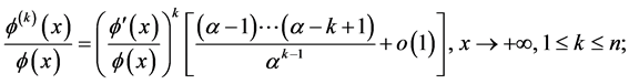
The second counterexample above shows that the set of relations in (3.5) in themselves do not grant that all the involved derivatives be regularly varying: it may well occur an abrupt transition from regular variation to rapid variation at a certain order of derivation. This is the main motivation for our Definition 3.1. But the asymptotic relations for are most important in applications and in this subsection we report three characterizations of these relations encountered in the literature and valid for any: the first deals with the derivatives of the ratio in (2.3), , and is used in the monograph by Lantsman [9] ; the second is a slight variant dealing with the derivatives of the logarithmic derivative; the third highlights the behavior at of the derivatives of the associated function. This last characterization is a nontrivial and useful result proved by Balkema, Geluk and de Haan ( [7] ; Lemma 9, p. 410) using an ingenious device.

Proposition 3.2. (Several characterizations). For an large enough, the following four sets of asymptotic relations, for a fixed, are equivalent to each other:

(3.21)

(3.22)

(3.23)

(3.24)

The reader will notice in the proof that the differential expressions “” stem out from successive differentiations of.

Proof. We use notation. To prove “(3.22) Û (3.23)” we use the identity

(3.25)

from which, putting, the equivalence easily follows for. By induction suppose the equivalence true for a certain; (3.22) true for imply the relations in (3.23) true for whereas (3.25), for, yields

(3.26)

which implies the relation in (3.23) for. Viceversa, if (3.23) are true for then the relations in (3.23) are true for whereas, for, we get from (3.25):

(3.27)

the sum in square brackets being. Let us now consider the obvious relations concerning the function defined in (3.24) and valid for all:

(3.28)

The equivalence (3.22) Û (3.24) is contained in the following:

(3.29)

First, it is elementary to prove by induction the formula

(3.30)

wherein, and the explicit expressions of the coefficients are not needed except for. If the set of relations on the left in (3.29) holds true then (3.30) at once implies the validity of the set on the right whereas we proceed by induction to prove the converse inference. Let the set of relations on the right in (3.29) holds true with k replaced by, then the inductive assumption grants all relations on the left in (3.29). Now we consider (3.30) with k replaced by, and solve it with respect to so getting

(3.31)

having used the relation in (3.29) for and. The last and most difficult equivalence is “(3.21)Û (3.24)” a direct proof of which via Faà di Bruno’s formula would involve cumbersome calculations. We report the original proof in a somewhat simplified form explicitly writing the arguments of the involved functions, avoiding the use of a change of variable, and with some additional passages to motivate the technical ideas of the proof. From representation, by direct routine differentiation and factoring out common factors, we get

(3.32)

wherein we have used the expression of to get the final expression of and the expression of to get the final expression of. It is clear that further differentiations yield expressions for the operators

(3.33)

and we shall prove the following representation:

(3.34)

where is a polynomial in each term of which contains a factor with. This is true for and a simple proof by induction, provided by the authors of [7] , is based on an equation linking simply obtained by differentiation of (3.33):

(3.35)

If now (3.34) is assumed true for a certain k then, differentiating both sides and using (3.35) in the left-hand side, we get

(3.36)

whence

(3.37)

where we have put

(3.38)

the right-hand side being a polynomial in each term of which contains a factor with, and this proves (3.34) for. Starting from (3.34) the proof by induction of the equivalence “(3.21) Û (3.24)” is quite trivial.,

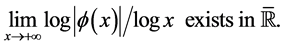
Balkema, Geluk and de Haan ( [7] ; p. 412) call “smoothly varying of exponent (º index)” a positive -function f defined on a neighborhood of such that the associated function satisfies the relations in (3.24) for all. In our context we give

Definition 3.2. (Smooth variation of higher order). A function large enough, is termed “smoothly varying at of order n and index” if the four equivalent properties in Proposition 3.2, referred to, are satisfied. We denote this class by: { of order n}.

Notice that in our definition is allowed to be either >0 or <0, the essential point being that it ultimately assumes only one strict sign. From Proposition 3.1-(II) and the examples (3.18)-(3.20) we get the following inclusions:

(3.39)

the reason of the strict inclusion being that some derivatives of a smoothly-varying function may vanish or change sign infinitely often. Examples:

(3.40)

In the third example all derivatives are rapidly varying whereas in the fourth example they have no index of variation at. Let us consider the further example of a function already exibited in (2.22):

(3.41)

If as in (3.24) we associate to the function it is easy to check the following:

(3.42)

In fact we have from whence an elementary induction proves the representation

(3.43)

implying for each if.

The anomalies in these examples make the definition of smooth variation a bit unsatisfying from a theoretical viewpoint unlike the definition of higher-order regular variation; they also show that the possible more complete locution “smooth regular variation” would not be appropriate; however it turns out that relations in (3.21)-(3.24), regardless of, are the right ones required in various applications. In the next proposition it is asserted that the derivative of a smoothly-varying function may not be smoothly-varying only if the index is zero whereas antiderivatives are always smoothly varying with suitable indexes.

Proposition 3.3. (Derivatives and integrals of smoothly varying functions). (I)

(3.44)

(II) If then

(3.45)

The very same inferences in the case of regular variation, i.e. with replaced by, are included in Propositions 2.4-(I), 2.6-(I) and Definition 3.1.

Proof. We report the more elementary arguments used in ( [8] ; Prop. 1.8.1, p. 44) in preference to those in ( [7] ; Lemmas 10-11, p. 412). For (3.44) put and notice that is ultimately of one strict sign as; hence for each we may write by (3.21):

(3.46)

To prove the first inference in (3.45) put. Recalling that has ultimately one strict sign and that “” Proposition 2.4-(I) implies and by (3.21) we have for each:

(3.47)

A similar proof in case of divergence.,

Notice that, with defined in (3.24), is recovered by the formula and that regular variation of may have ambiguous effects on. The reader may check that:

(3.48)

using “” and the estimates in (2.19) referred to. The case remains undecided as shown by:

(3.49)

(3.50)

To end this section let us ask ourselves what can be said about relations in (3.21) holding true with some unknown coefficients on the right and we give a result― needed in the sequel―concerning the circumstance.

Proposition 3.4. Let a function large enough, satisfy the following asymptotic relations:

(3.51)

(3.52)

for some unspecified constants. Then

Proof. The claim amounts to state that the’s coincide with the coefficients in (3.21). Now, if “” then Proposition 3.1-(II) states the stronger assertion “” and, moreover, for there is nothing further to be proved. On the contrary if for some coefficient is zero then our claim will be proved once we show that all the successive coefficients are zero as well. In fact if “” and “” for some, then:

(3.53)

(3.54)

using (3.51) and then the secod relation in (3.53)

(3.55)

hence and the proof is over. Note in passing that the second circumstance implies “” as the two relations in (3.53) imply:

(3.56)

,

4. The Theory of Higher-Order Rapid Variation

Before giving the proper definition of higher-order rapid variation it is good to add some remarks about the additional condition

(4.1)

appearing in Proposition 2.4-(II). The counterexample in (2.89) shows that this supplementary condition is almost necessary to obtain a meaningful general result about the asymptotic behavior of the antiderivatives of a rapidly-varying function. Now if in (2.84)-(2.85) we put, with the proper choice of, then the asymptotic behavior of F can be reread as

(4.2)

and, changing again notation, we have one of the following two equivalent relations:

(4.3)

For some applications conditions like those in (4.3) are necessary for meaningful general results as, e.g., in determining asymptotic expansions of antiderivatives and in another class of expansions studied in Part II, §11, of this work: this justifies the following restricted concept of rapid variation.

Definition 4.1. (Rapid variation of higher order).

(I) (First order). A function is called “rapidly varying at (of order 1) in the strong restricted sense” if

(4.4)

(II) (Higher order). A function is called “rapidly varying at of order in the strong restricted sense” if all the functions are rapidly varying at in the strong restricted sense and this amounts to say that the following conditions hold true as:

(4.5)

(4.6)

(4.7)

If is rapidly varying at of order in the previous strong restricted sense then, by (2.106), all the functions belong to the same class, either or, hence we shall use notation to denote that enjoys the properties in (4.5)-(4.6)-(4.7) plus the corresponding value of the limit in (2.2). In most cases we shall not be interested in functions satisfying (4.5)-(4.6) but not (4.7), and so we use no additional notation to highlight the “strong restricted sense”.

Remarks. 1. According to our definitions when we speak of a function rapidly varying (without specifying the order) we are using Definition 2.1 meaning that: for x large enough and (2.2) holds true. But when we speak of a function rapidly varying of order 1 (usually omitting the additional locution “in the strong restricted sense”) we are using the stronger Definition 4.1.

2. Conditions in (4.7) obviously imply those in (4.6) whereas, viceversa, complicated calculations in the attempt of proving (4.7) in addition to (4.6) may be usually saved using the classical result (already mentioned in the proof of Proposition 2.5) that: “”. For instance (4.5)- (4.7) are trivially satisfied for the functions listed in (2.8) which are the most common functions rapidly varying at of any order in our strong restricted sense.

As concerns the analogue of Proposition 3.1 it happens that relations in (3.5) have no analogues for rapidly-varying functions of higher order whereas those in (3.6) have so yielding a useful characterization of this class of functions.

Proposition 4.1. (Principal parts of higher derivatives in case of rapid variation). Let and conditions in (4.5) be satisfied; then , i.e. conditions in (4.7) hold true, if and only if the following four equivalent sets of conditions are satisfied:

(4.8)

(4.9)

(4.10)

(4.11)

It follows that even for almost all x large enough. Relations in (4.10) are formally obtained from those in (3.6) as the index tends to. Relations in (4.10) imply the following asymptotic scale:

(4.12)

whereas a different way of writing relations in (4.6) would give the weaker scale:

(4.13)

Proof. Relations in (4.9) and in (4.11) simply are different ways of rewriting relations respectively in (4.8) and in (4.10). Now inspecting (4.7) we have for:

(4.14)

which is (4.9) and (4.10) for. Moreover, for any we have

(4.15)

hence (4.7) are equivalent to (4.9). It remains to prove the equivalence between (4.9) and (4.10) for and. Supposing relations in (4.9) true we start from the asymptotic relation involving and replace in the right-hand side with the analogous relation while leaving unaltered; so we get

(4.16)

If this gives which is (4.10) for. If we reapply the procedure to the last expression in (4.16) so getting

(4.17)

If this gives which is (4.10) for; and if we repeat the procedure and get all relations in (4.10). Viceversa suppose (4.10) true and assume, by induction, that they imply (4.9), i.e. (4.8), for k ranging in for some, as this is trivially true for. Let us write down the relations in (4.10) for:

(4.18)

(4.19)

Using (4.18) and the relation in (4.8) involving the ratio, which is true by the inductive hypothesis, we get

(4.20)

which is the relation in (4.9) for and the proof is over.,

An instructive counterexample concerning Definition 4.1 and the associated function. Let us consider the following function

(4.21)

wherein ultimately “”, whereas changes sign infinitely often though being bounded. The relations hold true:

(4.22)

whence we infer that

(4.23)

and condition (4.1) is not satisfied as

(4.24)

and does not exist. So for any we have an example of a function f such that:

(4.25)

though for the additional property “bounded” is satisfied.

For we also have an example of a function f such that:

(4.26)

As concerns the associated function in (3.24), , the second formula in (3.32) yields

(4.27)

Hence for any we have an example of a function satisfying the special additional relation, and also for, such that the associated function has a second derivative oscillatory and unbounded. This shows that the properties of the associated function have little meaning, if any, in the context of rapid variation.

A remark about the ratios. In Definition 4.1-(II) relations in (4.6) imply the following chain:

(4.28)

A remark about. If a function with ultimately, satisfies condition

(4.29)

an integration yields

(4.30)

Moreover the identity in (4.14) gives

(4.31)

i.e. with according to Proposition 2.6. In conclusion (4.29) implies “”. Thus, if the asymptotic relation in (4.29) holds true for some real number and if it is known that, then it must be. Analogously, using the identity in (4.15) and under the regularity assumptions in Proposition 4.1, we prove that if

(4.32)

then

(4.33)

and

(4.34)

i.e. with. Hence if it is known a priori that for some then. This fact will be needed in the sequel.

Corollary 4.2. (Summing up the behaviors of the higher derivatives). Let,. Then, as:

(4.35)

(4.36)

(4.37)

(4.38)

Examples.

(4.39)

5. Asymptotic Functional Equations for Regular or Rapid Variation

Using representations in (2.12) it is easy to prove certain useful asymptotic relations satisfied by regularly-varying functions and in particular (2.6) which has been assumed by Karamata as the definition of a general concept of regular variation. The standpoint in this section is that of highlighting how a given function acts upon various asymptotic relations and we give these properties the collective name of “asymptotic functional equations”.

Proposition 5.1. (Slow and regular variation). (I) A function enjoys the following asymptotic property:

(5.1)

which states that a slowly-varying function transforms the relation of “asymptotic similarity between functions diverging to”, see (1.11), into the stronger relation of “asymptotic equivalence”: A property elementarily checked for the iterated logarithms and their powers. In particular satisfies the asymptotic functional equation:

(5.2)

which, by the presence of the parameter, says a bit more than “preserving asymptotic equivalence”.

(II) A function enjoys the following asymptotic properties:

(5.3)

(5.4)

They mean that a regularly-varying function preserves the relations of “asymptotic similarity” and “asymptotic equivalence” between functions diverging to with an addditional property concerning the multiplication of the argument by a constant factor. The last inference may be symbolically written as the asymptotic functional equation:

(5.5)

in particular:

(5.6)

The asymptotic functional equation (2.6) is a special case of (5.6) and it expresses the “power-like” type of growth of. For we have the more precise result:

(5.7)

referring to §11 in Part II for expansions with more terms. Two special cases of (5.7) are:

(5.8)

(5.9)

Another useful consequence of (5.6) is:

(5.10)

and in particular:

(5.11)

Proof. Rewrite (2.12) as

(5.12)

To prove (5.1) and (5.3) let be two functions defined on a neighborhood of such that:

(5.13)

then

(5.14)

By (5.13):

(5.15)

and

(5.16)

so that

(5.17)

For we use these facts in the right-hand side of (5.14) so getting the inequalities

(5.18)

which are the precise meaning of the thesis in (5.3). And for the more precise relation in (5.1) is obtained. Analogously we have

(5.19)

which is (5.4), equivalent to (5.5). The asymptotic expansion in (5.7) is similarly proved:

(5.20)

Last, (5.10) follows from the mean-value theorem of integral calculus:

(5.21)

as “”. An alternative proof, only valid for, follows from (5.7) applied to an antiderivative of, say, which satisfies, by writing

(5.22)

and then using (2.78) or (2.79).,

A comment on uniform convergence. Refining the calculations in (5.19) the last expression in (5.19) may be replaced by

(5.23)

where the symbols “” stand for suitable functions not dependent on. Hence:

(5.24)

and it is easily seen that the quantity on the right tends to zero, as, uniformly with respect to varying on any compact interval of type. This fact, elementary for regular variation in the strong sense, is a nontrivial result for regular variation in Karamata’s sense, basic for the whole theory: Uniform Convergence Theorem ( [8] ; pp. 6-10 and pp. 22-23). A minor result in the general theory states that the asymptotic functional equation (2.6) is equivalent to the (seemingly more general) (5.6).

In the next proposition special cases of the asymptotic relation in (5.7) are commented upon.

Proposition 5.2. (I) (Asymptotic sublinearity). If then (2.19) implies that and (5.8) becomes:

(5.25)

a property enjoyed by all functions such that, as follows at once from representation

(5.26)

Such a property may be interpreted as a kind of “asymptotic sublinearity”.

(II) (Asymptotic linearity). For a function and the asymptotic functional equation in (5.9) becomes:

(5.27)

a property enjoyed by all functions such that , as again follows from representation (5.26). An instance is provided by the function defined in (3.24) and associated to in defining the concept of smooth variation. (As we know, the sole condition implies “regularly varying at of index 1 in the general sense of Karamata”.)

The property in (5.27) may be interpreted as a kind of “asymptotic linearity”. For (5.27) takes the form:

(5.28)

an equation satisfied by all functions such that , a meaningful subclass being that of the functions ultimately “positive and concave”. A proper label for the property in (5.28) is “asymptotic uniform continuity at” as it can be proved that:

“A function is uniformly continuous on iff it is continuous on and asymptotically uniformly continuous at”.

(III) (A subclass of slowly-varying functions). The strong asymptotic functional equation

(5.29)

states that transforms the relation of “asymptotic equivalence between functions diverging to” into the stronger relation of “asymptotic equivalence with an infinitesimal remainder”. Representation in (5.26) easily implies that (5.29) is satisfied by any such that, for instance by all functions “and bounded” and by:

(5.30)

but neither by nor by.

For rapid variation, which formally refers to the limit cases of regular variation, only a formal analogue of (5.5) holds true.

Proposition 5.3. (Rapid variation). (I) If and if then:

(5.31)

In particular

(5.32)

(II) If and if then:

(5.33)

In particular

(5.34)

The asymptotic functional relations (5.32) and (5.34) where assumed by de Haan as definitions of the general classes of (measurable) rapidly-varying functions of index, respectively: ( [8] ; p. 83).

Proof. (I) From relation (2.2) we get that such that implies “”, and for all x large enough we also have:

(5.35)

(5.36)

whence

(5.37)

The limits in (5.31) follow by applying the exponential as in (5.19) and those in (5.33) follow by applying the just-proved result to the function.,

Conflicts of Interest

The authors declare no conflicts of interest.

References

[1]	Granata, A. (2011) Analytic Theory of Finite Asymptotic Expansions in the Real Domain. Part I: Two-Term Expansions of Differentiable Functions. Analysis Mathematica, 37, 245-287. http://dx.doi.org/10.1007/s10476-011-0402-7
[2]	Granata, A. (2015) The Factorizational Theory of Finite Asymptotic Expansions in the Real Domain: A Survey of the Main Results. Advances in Pure Mathematics, 5, 1-20. http://dx.doi.org/10.4236/apm.2015.51001
[3]	Granata, A. (2015) Analytic Theory of Finite Asymptotic Expansions in the Real Domain. Part II-A: The Factorizational Theory for Chebyshev Asymptotic Scales. Advances in Pure Mathematics, 5, 454-480. http://dx.doi.org/10.4236/apm.2015.58045
[4]	Granata, A. (2015) Analytic Theory of Finite Asymptotic Expansions in the Real Domain. Part II-B: Solutions of Differential Inequalities and Asymptotic Admissibility of Standard Derivatives. Advances in Pure Mathematics, 5, 481-502. http://dx.doi.org/10.4236/apm.2015.58046
[5]	Granata, A. (2015) Analytic Theory of Finite Asymptotic Expansions in the Real Domain. Part II-C: Constructive Algorithms for Canonical Factorizations and a Special Class of Asymptotic Scales. Advances in Pure Mathematics, 5, 503-526. http://dx.doi.org/10.4236/apm.2015.58047
[6]	Bourbaki, N. (1976) Fonctions d’une Variable Réelle-Théorie élémentaire. Hermann, Paris.
[7]	Balkema, A.A., Geluk, J.L. and de Haan, L. (1979) An Extension of Karamata’s Tauberian Theorem and Its Connection with Complementary Convex Functions. The Quarterly Journal of Mathematics, Oxford University Press, Series 2, 30, 385-416. http://dx.doi.org/10.1093/qmath/30.4.385
[8]	Bingham, N.H., Goldie, C.M. and Teugels, J.L. (1987) Regular Variation. Cambridge University Press, Cambridge. http://dx.doi.org/10.1017/CBO9780511721434
[9]	Lantsman, M.H. (2001) Asymptotics of Linear Differential Equations. Springer Science+ Business Media, Dordrecht. http://dx.doi.org/10.1007/978-94-015-9797-5
[10]	Seneta, E. (1976) Regularly Varying Functions. Springer-Verlag, Berlin-Heidelberg-New York. http://dx.doi.org/10.1007/BFb0079658
[11]	Pólya, G. and Szëgo, G. (1972) Problems and Theorems in Analysis. Vol. I. Springer-Verlag, Berlin-Heidelberg-New York. http://dx.doi.org/10.1007/978-1-4757-1640-5
[12]	Granata, A. (2010) The Problem of Differentiating an Asymptotic Expansion in Real Powers. Part I: Unsatisfactory or Partial Results by Classical Approaches. Analysis Mathematica, 36, 85-112. http://dx.doi.org/10.1007/s10476-010-0201-6
[13]	Granata, A. (2015) The Role of Asymptotic Mean in the Geometric Theory of Asymptotic Expansions in the Real Domain. Advances in Pure Mathematics, 5, 100-119. http://dx.doi.org/10.4236/apm.2015.52013